Battery pack during thermal runaway

Note

The script and BDF file for this example can be found under the examples/battery/ directory.

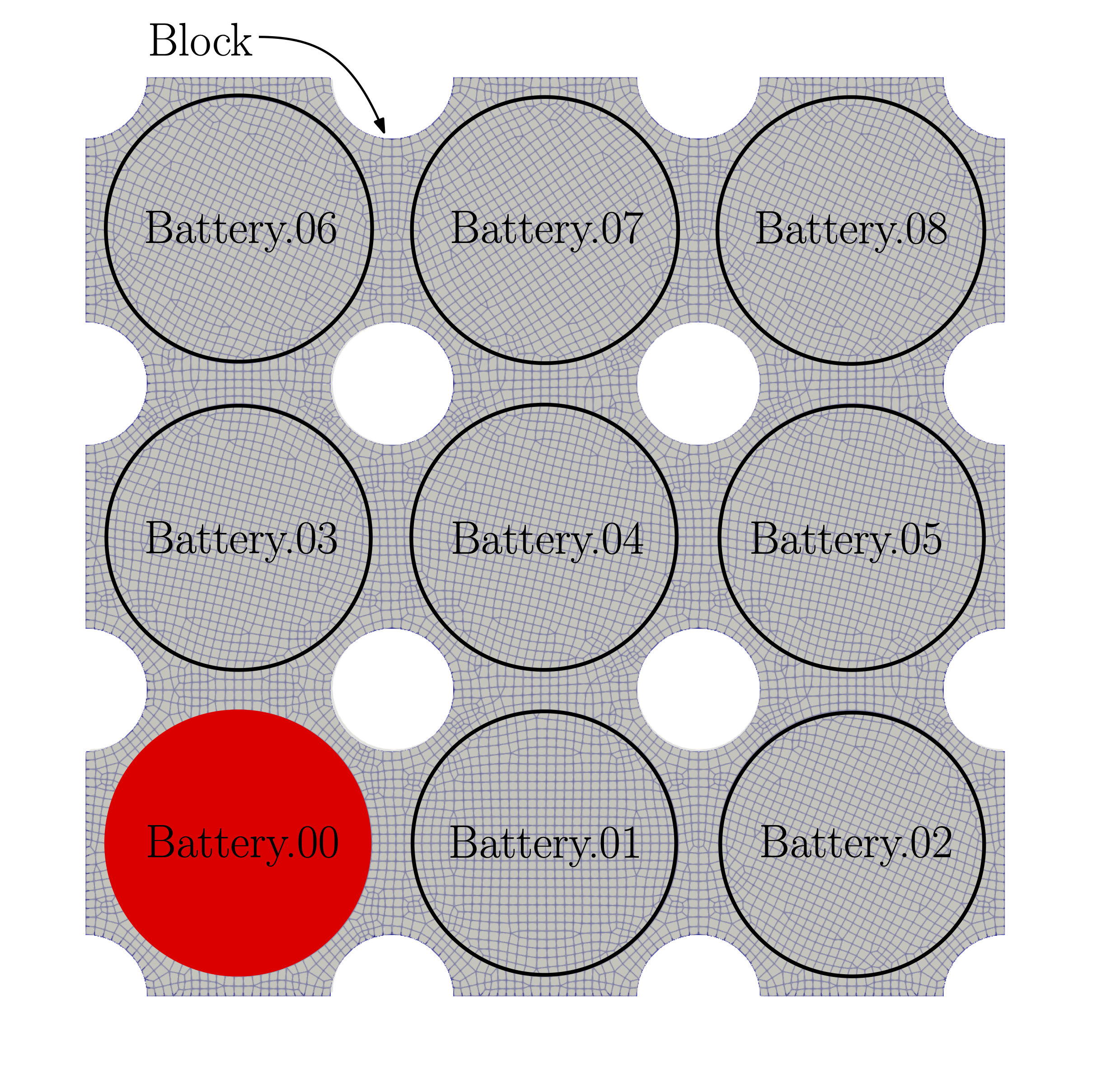
This example demonstrates transient heating of a battery pack with one cell undergoing thermal runaway. The domain is an aluminum battery pack with 9 cylindrical cells embedded in a grid-pattern. The cell in the corner undergoes thermal runaway, releasing a large amount of heat for 2 seconds. The heat conduction of the battery pack is then computed for 5 seconds in total. The maximum temperature within a cell is computed over all time steps. This is done for 3 cells: the cell undergoing thermal runaway, the nearest cell adjacent to it, and the cell on the diagonal near it. Computing the maximum temperature of these cells could be used to prevent other cells in the pack from going into thermal runaway, leading to a cascading failure. The problem domain is shown in the figure below with the BDF component names labeled.

This example will demonstrate a number of useful pyTACS features, including:

• Transient heat conduction physics

• Two materials modeled in the same mesh

• Time-specified loading: the right-hand-side is given as a user-defined function of time

• Evaluating multiple functions in different regions

• Easy domain-selection enabling the previous three items

First, import required libraries:

import os
from pprint import pprint

import numpy as np
from mpi4py import MPI

from tacs import functions, constitutive, elements, TACS, pyTACS

Import the bdf file, initialize the pyTACS object, and define the mateterial properties for the problem. This problem uses two different materials: one material for the battery cells, and aluminum material propertiesfor the battery pack.

# Name of the bdf file to get the mesh
bdfFile = os.path.join(os.path.dirname(__file__), 'battery_pack.bdf')

# Instantiate the pyTACS object
FEAAssembler = pyTACS(bdfFile, comm)

# Specify the plate thickness
tplate = 0.065

# Define material properties for two materials used in this problem
# Properties of the battery cells
battery_rho = 1460.0  # density kg/m^3
battery_kappa = 1.3 # Thermal conductivity W/(m⋅K)
battery_cp = 880.0 # Specific heat J/(kg⋅K)

# Properties of the battery pack (aluminum)
alum_rho = 2700.0  # density kg/m^3
alum_kappa = 204.0 # Thermal conductivity W/(m⋅K)
alum_cp = 883.0 # Specific heat J/(kg⋅K)

Next, set up the elemCallBack() function. By checking the compDescript value, the elements are set with either aluminum material properties, or battery material properties.

# The callback function to define the element properties
def elemCallBack(dvNum, compID, compDescript, elemDescripts, globalDVs, **kwargs):

    # Set up property and constitutive objects
    if compDescript == 'Block':  # If the bdf file labels this component as "Block", then it is aluminum
        prop = constitutive.MaterialProperties(rho=alum_rho, kappa=alum_kappa, specific_heat=alum_cp)
    else:  # otherwise it is a battery
        prop = constitutive.MaterialProperties(rho=battery_rho, kappa=battery_kappa, specific_heat=battery_cp)

    # Set one thickness value for every component
    con = constitutive.PlaneStressConstitutive(prop, t=tplate, tNum=-1)

    # For each element type in this component,
    # pass back the appropriate tacs element object
    elemList = []
    model = elements.HeatConduction2D(con)
    for elemDescript in elemDescripts:
        if elemDescript in ['CQUAD4', 'CQUADR']:
            basis = elements.LinearQuadBasis()
        elif elemDescript in ['CTRIA3', 'CTRIAR']:
            basis = elements.LinearTriangleBasis()
        else:
            print("Element '%s' not recognized" % (elemDescript))
        elem = elements.Element2D(model, basis)
        elemList.append(elem)

    return elemList

# Set up constitutive objects and elements
FEAAssembler.initialize(elemCallBack)

Next, define the instance of TransientProblem, give it a name (in this case, we've called it "Transient"), and declare the initial time, tInit, final time, tFinal, and the number of time steps, numSteps.

# Create a transient problem that will represent time-varying heat conduction
transientProblem = FEAAssembler.createTransientProblem('Transient', tInit=0.0, tFinal=5.0, numSteps=50)

Here we define the time-varying heat flux for this problem. This simulates one battery going into thermal runaway and releasing a large amount of heat for 2 seconds. To do this, we first get all of the problem's time steps using TransientProblem.getTimeSteps. Then, we loop through each time step, and add a heat-flux for each time step where the time is less than or equal to 2 seconds. To add the heat flux only to elements corresponding to the battery undergoing thermal runaway, we use the pyTACS.selectCompIDs method. Those component IDs are then passed as an input when we define the load using the TransientProblem.addLoadToComponents method, which takes as input the time-step, the component IDs that we just selected, and an array specifiying the total load to apply, which will be spread out over all elements in the specified components. Since the heat transfer problem has only one degree of freedom, this is an array of length 1. The value of 6000.0 used here indicates a total heat of 6000 Watts to be applied for 2 seconds, corresponding to 12,000 Joules of total thermal energy released by the battery during thermal runaway.

# Get the time steps and define the loads
timeSteps = transientProblem.getTimeSteps()
for i, t in enumerate(timeSteps):
    if t <= 2.0:  # only apply the load for the first 2 seconds (step function)
        # select the component of the battery undergoing thermal runaway
        compIDs = FEAAssembler.selectCompIDs(include=["Battery.00"])

        # Define the heat-flux: apply 6000 Watts spread out over the face of the cell undergoing thermal runaway
        transientProblem.addLoadToComponents(i, compIDs, [6000.0])

Next, we define the functions that we want to evaluate for this problem. In this case, we are interested in the maximum temperature of the cell undergoing thermal runaway, as well as the maximum temperature of the two cells closest to it to prevent them from exceeding their maximum operting temperature, preventing a cascading thermal runaway event. To do this, we first select the component IDs for each of these three batteries using the same procedure that was used to define the heat flux.

# Define the functions of interest as maximum temperature withing 3 different batteries
compIDs_00 = FEAAssembler.selectCompIDs(["Battery.00"])  # battery undergoing thermal runaway
compIDs_01 = FEAAssembler.selectCompIDs(["Battery.01"])  # adjecent battery
compIDs_04 = FEAAssembler.selectCompIDs(["Battery.04"])  # diagonal battery

With the component IDs for each cell selected, we can define the functions using the TransientProblem.addFunction method. This method takes as input a user-defined name for this function, and an uninitialized TACS functions class, which in this case is KSTemperature. Two keyword arguments used here: first, ksWeight, corresponding to the "rho" value in the KS-aggregation function, and the second, compIDs, where we pass in the component IDs for each battery that we just selected. The KS function in the transient case computes the approximate maximum over all time steps and all elements in the specified domains.

transientProblem.addFunction('ks_temp_corner', functions.KSTemperature,
                             ksWeight=100.0, compIDs=compIDs_00)
transientProblem.addFunction('ks_temp_adjacent', functions.KSTemperature,
                             ksWeight=100.0, compIDs=compIDs_01)
transientProblem.addFunction('ks_temp_diagonal', functions.KSTemperature,
                             ksWeight=100.0, compIDs=compIDs_04)

Now that our problem has been set up with loads and functions we can solve it and evaluate its functions using the TransientProblem.solve and TransientProblem.evalFunctions methods, respectively.

funcs = {}
transientProblem.solve()
transientProblem.evalFunctions(funcs)

To get the function sensitivity with respect to the design variables and node locations using the TransientProblem.evalFunctionsSens method.

funcsSens = {}
transientProblem.evalFunctionsSens(funcsSens)

Finally, we can write out our solution to an f5 file format for further post-processing and visualization by using the TransientProblem.writeSolution method.

transientProblem.writeSolution()

This produces several files called Transient_000_000.f5 through Transient_000_050.f5 in our runscript directory. The first index after the problem name indicates the optimization step (000 in this case for a single solve), and the second index indicates the time-step of the analysis (000 through 050). These files can be converted into a .vtk file (using f5tovtk) for visualization in Paraview or a .plt (using f5totec) for visualization in TecPlot using:

$ f5tovtk Transient_000_*.f5

or

$ f5totec Transient_000_*.f5

The animation below shows what the transient heat transfer temperature solution looks like when visualized in Paraview.