Plate under static load
Note
The script for this example can be found under the examples/plate/ directory.
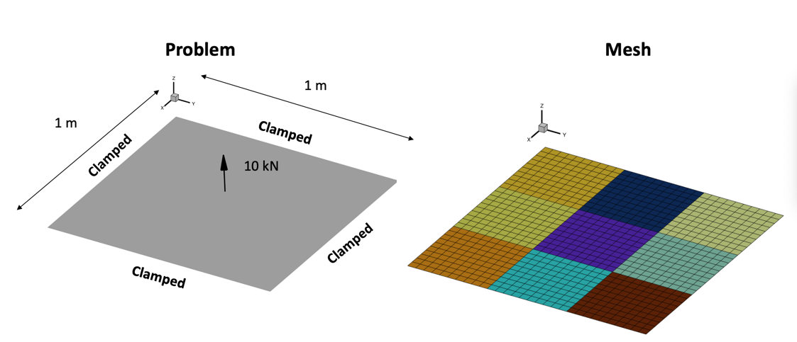
This problem will show how to use some of pytacs more advanced load setting procedures. The nominal case is a 1m x 1m flat plate. The perimeter of the plate is fixed in all 6 degrees of freedom. The plate comprises 900 CQUAD4 elements. We consider a static case where a 10 kN point force is applied at the plate center.
First, import required libraries:
import numpy as np
from tacs import functions, constitutive, elements, pyTACS
Next, we must create the pyTACS class.
pyTACS acts as an assembler for all of the TACS submodules.
It's purpose is to read in mesh files, setup TACS element objects, and create TACS problems for analysis.
To create a pyTACS class, at minimum, a NASTRAN bdf defining nodes, elements, and boundary conditions is required.
bdfFile = './plate.bdf'
FEAAssembler = pyTACS(bdfFile)
Next step, we must initialize pyTACS.
pyTACS must always be initialized before an analysis can be conducted.
During this step, TACS element objects and design variables are setup and assigned for use in analysis.
There are two ways to call the pyTACS.initialize method.
The first, involves defining a elemCallBack() function that tells pyTACS which TACS element to setup
for each NASTRAN element card in the BDF and passing this function handle to the pyTACS.initialize.
The second method, allows pyTACS to automatically initialize itself based on information from the BDF file,
as long as property cards exist for every element. This is done by calling the
pyTACS.initialize method with no arguments.
For more information on the pyTACS initialization procedure, see here.
For this example, we will take the first approach. Our elemCallBack() for this model is defined below.
def elemCallBack(dvNum, compID, compDescript, elemDescripts, specialDVs, **kwargs):
    # Material properties
    rho = 2500.0        # density kg/m^3
    E = 70e9            # Young's modulus (Pa)
    nu = 0.3            # Poisson's ratio
    ys = 464.0e6        # yield stress

    # Plate geometry
    tplate = 0.005    # 5 mm

    # Set up material properties
    prop = constitutive.MaterialProperties(rho=rho, E=E, nu=nu, ys=ys)
    # Set up constitutive model
    con = constitutive.IsoShellConstitutive(prop, t=tplate, tNum=dvNum)
    # Set the transform used to define shell stresses, None defaults to NaturalShellTransform
    transform = None
    # Set up tacs element for every entry in elemDescripts
    # According to the bdf file, elemDescripts should always be ["CQUAD4"]
    elemList = []
    for descript in elemDescripts:
        if descript == 'CQUAD4':
            elem = elements.Quad4Shell(transform, con)
        else: # Add a catch for any unexpected element types
            raise ValueError(f"Unexpected element of type {descript}.")
    return elemList
The callback function for this example is pretty simple.
First, we define the MaterialProperties for aluminum.
We then use those properties and the plate thickness to setup a IsoShellConstitutive
for modeling the shell stiffness. We set the element transform type to None. Finally, for every element card in
elemDescripts, we pass back an appropriate initialized TACS element class. In this case, the only element type
in the BDF are CQUAD4, so we'll always pass back an elemList with one entry, a Quad4Shell.
Now that the callback function has been defined, we can pass it to pyTACS.initialize.
FEAAssembler.initialize(elemCallBack)
The pyTACS has been initialized, we can now use it to create a StaticProblem.
TACS problem classes are generally responsible for setting loads, solving analyses, evaluating
functions of interests, and computing gradients.
To create our StaticProblem we can use the
pyTACS.createStaticProblem method.
This method requires at minimum a name for our problem.
staticProb = FEAAssembler.createStaticProblem('point_force')
Next, we'll add some functions of interest to our problem that we can evaluate after we've solved it.
This can be accomplished using StaticProblem.addFunction method.
This method takes a user-defined name and any uninitialized TACS functions class as an input. Additional arguments necessary to
setup the function class (minus the Assembler) can be passed as keyword arguments to StaticProblem.addFunction.
For now let's add a function to evaluate the mass of the plate using StructuralMass
and a function to evaluate the maximum vonMises-based failure criteria using KSFailure.
staticProb.addFunction('mass', functions.StructuralMass)
staticProb.addFunction('ks_vmfailure', functions.KSFailure, ksWeight=100.0)
Now let's add our point load to the problem. We can do this by using the
StaticProblem.addLoadToNodes method and
selecting node ID 481 (the node at the center of the plate).
F = np.array([0.0, 0.0, 1e4, 0.0, 0.0, 0.0])
staticProb.addLoadToNodes(481, F, nastranOrdering=True)
Now that our problem has been setup with loads and functions we can solve it and evaluate its functions using the
StaticProblem.solve and
StaticProblem.evalFunctions methods, respectively.
funcs = {}
staticProb.solve()
staticProb.evalFunctions(funcs)
To get the function sensitivity with respect to the design variables and node locations using the
StaticProblem.evalFunctionsSens method.
funcsSens = {}
staticProb.evalFunctionsSens(funcsSens)
Finally, we can write out our solution to an f5 file format for further post-processing and visualization by using the
StaticProblem.writeSolution method.
staticProb.writeSolution()
This produces a file called point_force_000.f5 in our runscript directory. This file can be converted into a .vtk file
(using f5tovtk) for visualization in Paraview or a .plt (using f5totec) for visualization in TecPlot using:
$ f5tovtk point_force_000.f5
or
$ f5totec point_force_000.f5
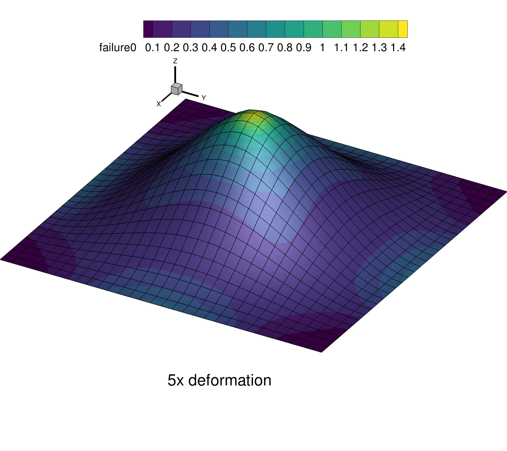
The figure below shows what the failure contour mapped over the deformed plate looks as visualized in Tecplot.