The Brachistochrone Problem

The brachistochrone problem is a classic problem in the calculus of variations, first posed by Johann Bernoulli in 1696. The name comes from the Greek words brachistos (shortest) and chronos (time). The problem asks: given two points at different heights, what is the path along which a particle will slide from the higher point to the lower point in the shortest time, under the influence of gravity alone?

Remarkably, the solution is not a straight line but a cycloid curve. This problem is fundamental in optimal control theory and serves as an excellent benchmark for trajectory optimization methods.

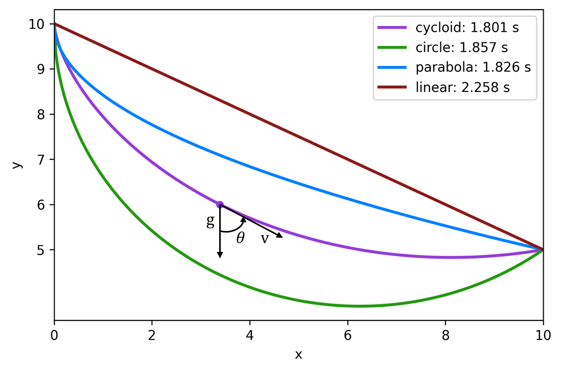
Figure 1. Brachistochrone optimal trajectory from point A to point B.

Problem Formulation

The objective is to minimize the travel time from an initial point $(x_0, y_0)$ to a final point $(x_f, y_f)$:

$$\min_{t_f, \theta(t)} \quad t_f$$

The state vector $\mathbf{q} = [x, y, v]^T$ represents the particle's horizontal position, vertical position, and velocity along the path. The control variable $\theta(t)$ is the angle of the tangent to the path with respect to the horizontal.

Dynamics

The particle dynamics under gravity are described by:

$$\begin{aligned} \dot{x} &= v \sin \theta \\ \dot{y} &= -v \cos \theta \\ \dot{v} &= g \cos \theta \end{aligned}$$

where $g = 9.80655 \, \text{m/s}^2$ is the gravitational acceleration, and $\theta$ is the path angle measured from the vertical downward direction.

Boundary Conditions

For this example, we use the following boundary conditions:

Initial conditions at $t = 0$:

$$\begin{aligned} x(0) &= 0 \\ y(0) &= 10 \\ v(0) &= 0 \end{aligned}$$

Final conditions at $t = t_f$:

$$\begin{aligned} x(t_f) &= 10 \\ y(t_f) &= 5 \end{aligned}$$

The final velocity is free (unconstrained), as we only require the particle to reach the target position.

Implementation in Amigo

The brachistochrone problem is solved using Amigo's direct transcription approach. The continuous-time optimal control problem is discretized into a nonlinear programming (NLP) problem using collocation.

Key Components

The problem is structured using several components:

1. ParticleDynamics: Enforces the particle dynamics equations relating the state derivatives to the state and control
2. TrapezoidRule: Implements trapezoidal integration to connect states between time steps
3. InitialConditions: Enforces the starting position and velocity
4. FinalConditions: Enforces the target endpoint
5. Objective: Minimizes the final time $t_f$

Model Structure

The model discretizes the trajectory into 100 time steps, creating design variables for the state at each node and control variables at each point. The components are linked together to form a sparse nonlinear programming problem that is efficiently solved using Amigo's interior-point optimizer.

import amigo as am
import numpy as np

# Time discretization
num_time_steps = 100

# Create and configure the model
model = am.Model("brachistochrone")

# Add component instances
model.add_component("dynamics", num_time_steps + 1, ParticleDynamics())
model.add_component("trap", 3 * num_time_steps, TrapezoidRule())
model.add_component("obj", 1, Objective())
model.add_component("ic", 1, InitialConditions())
model.add_component("fc", 1, FinalConditions())

# Link state variables for time integration
for i in range(3):
    start = i * num_time_steps
    end = (i + 1) * num_time_steps
    model.link(f"dynamics.q[:{num_time_steps}, {i}]", f"trap.q1[{start}:{end}]")
    model.link(f"dynamics.q[1:, {i}]", f"trap.q2[{start}:{end}]")
    model.link(f"dynamics.qdot[:-1, {i}]", f"trap.q1dot[{start}:{end}]")
    model.link(f"dynamics.qdot[1:, {i}]", f"trap.q2dot[{start}:{end}]")

# Link boundary conditions
model.link("dynamics.q[0, :]", "ic.q[0, :]")
model.link(f"dynamics.q[{num_time_steps}, :]", "fc.q[0, :]")
model.link("obj.tf[0]", "trap.tf")

# Initialize and solve
model.initialize()
x = model.create_vector()

# Set initial guess (straight line interpolation)
N = num_time_steps + 1
x["dynamics.q[:, 0]"] = np.linspace(0.0, 10.0, N)  # x position
x["dynamics.q[:, 1]"] = np.linspace(10.0, 5.0, N)  # y position
x["dynamics.q[:, 2]"] = np.linspace(0.0, 9.9, N)   # velocity
x["obj.tf"] = 3.0  # initial guess for final time

# Set bounds
lower = model.create_vector()
upper = model.create_vector()
lower["obj.tf"] = 1.0
upper["obj.tf"] = float("inf")
lower["dynamics.theta"] = 0.0
upper["dynamics.theta"] = np.pi

# Solve the optimization problem
opt = am.Optimizer(model, x, lower=lower, upper=upper)
opt.optimize({"max_iterations": 500})

print(f"Optimized final time: {x['obj.tf'][0]:.6f} s")

Results

The optimizer finds the optimal cycloid trajectory that minimizes travel time. The analytical solution for this specific problem configuration yields a time of approximately 1.86 seconds, which the numerical method closely matches.

Source Code

The complete implementation can be found in the examples/brachistochrone directory of the Amigo repository.

References

1. Bernoulli, J. (1696). "Problema novum ad cujus solutionem Mathematici invitantur"
2. Betts, J. T. (2010). "Practical Methods for Optimal Control and Estimation Using Nonlinear Programming", SIAM