Euler-Bernoulli Beam Optimization

Amigo-based FEM integrated within OpenMDAO

Author: Jack Turbush

For this tutorial, two important functions of Amigo will be discussed: using Amigo to solve analysis problems (specifically the Finite Element Method), and using Amigo within another optimization framework OpenMDAO. Amigo’s GPU-accelerable capabilities allow for efficient, differentiated analysis when an optimization-centered formulation for the analysis is available, and the post optimality derivatives that Amigo can compute allow for easy implementation into an external optimization loop.

This example is based on the OpenMDAO example listed here: (https://openmdao.org/newdocs/versions/latest/examples/beam_optimization_example.html), where the compliance of a cantilever beam is minimized by varying element heights constrained by total volume. Instead of computing the displacements and derivatives using the FEM + adjoint method as described in the example, Amigo can be used to compute these using a potential energy minimization-based FEM formulation.

What OpenMDAO sees is an analysis component intaking design variables for single iteration and outputting a displacement vector, compliance calculation, volume, and derivatives. What is really happening is Amigo running a sub-optimization to simulate the beam deflection using the finite element method.

Problem Formulation

The objective is to minimize the compliance of a cantilever beam with a tip load. The beam is split into 50 elements, fixed on the left, and loaded in the negative y direction on the right. Each 1D element has four degrees of freedom corresponding to displacement vertically and rotationally, $v_i, \theta_i, v_{i+1}, \theta_{i+1}$ The beam element heights are the design variables.

$$\begin{split} \begin{array}{r c l} \text{minimize} & & f^T v \\ \text{with respect to} & & h \\ \text{subject to} & & \text{sum}(h) b L_0 = \text{volume} \end{array} \end{split}$$

In OpenMDAO and in traditional FEM codes, the displacements vector $v$ is computed using the relationship

$$Kv = f$$

where K is the stiffness matrix. Usually, inverting K (The adjoint method is then used to compute the gradient of the objective $f^Tv$ with respect to the beam height vector $h$.

In Amigo, the displacements vector $v$, along with $\nabla_{h}(f^Td)$, is computed by considering the variational formulation of the problem and computing the optimization directly. If not familiar, the variational formulation of the finite element method, the traditional $Ku=f$ formulation can be derived from the variational statement of a structure

$$\Pi_{total} = U+W\\ \delta \Pi = 0$$

where the stationarity condition $\delta \Pi =0$ is the crux of the variational formulation. Here, $U$ is strain energy of the system, and $W$ is work from the surroundings. Equivalently, the total potential energy of the system can be treated as a minimization problem. Assembling the total potential energy equation, if each element strain energy is computed, and the work from the applied tip load is added, the displacements for this problem can be found as such:

$$\begin{split} \begin{array}{r c l} \text{minimize} & & \Pi_{total}= \sum_{e=1}^{50} U_{e} +Fv\vert_{e = 50 (x = L_0)} \\ \text{with respect to} & & v \\ \end{array} \end{split}$$

where

$$U_{e} = \frac{1}{2}v_e^T K_ev_e$$

and

$$K_e = \frac{EI}{L_0^3} \begin{bmatrix} 12 & 6 L_0 & -12 & 6 L_0 \\ 6 L_0 & 4 L_0^2 & -6 L_0 & 2 L_0^2 \\ -12 & -6 L_0 & 12 & -6 L_0 \\ 6 L_0 & 2 L_0^2 & -6 L_0 & 4 L_0^2 \end{bmatrix}$$

where the element-wise stiffness matrix is shared with OpenMDAO’s logic.

Boundary Conditions

For this example, we will use the following boundary conditions:

• $v,\theta\vert_{x= 0} = 0$
• $F = -1$ (v direction)

Problem Setup

We begin by defining the physical parameters

length = 1.0
nelems = 50

x_coords = np.linspace(0, length, nelems + 1)

nodes = np.arange(nelems + 1, dtype=int)
conn = np.array([[i, i + 1] for i in range(nelems)], dtype=int)

Implementation

OpenMDAO Components

The following subsystems are added to call amigo and extract the objective, constraint, and derivatives.

1. indeps
2. fea

Key Amigo components

The problem is structured using several components:

1. beam_element
2. BoundaryCondition
3. AppliedLoad
4. NodeSource
5. Compliance
6. VolumeConstraint

Components

Component Group 1: Element Strain Energy

This component group calculates the displacement vector and the strain energy for the element, which is contributed to the objective function. There will be 50 elements in this group, each contributing an individual strain energy to the objective function.

class beam_element(am.Component):
    """
    Element Strain Energy for potential energy minimization.
    Equilibrium is obtained by minimizing total PE = Strain Energy - Work.
    No residuals needed - equilibrium comes from dPE/du = 0.
    """

    def __init__(self):
        super().__init__()
        self.add_input("v", shape=(2,), value=0.0)
        self.add_input("t", shape=(2,), value=0.0)
        self.add_data("h")
        self.add_constant("E", value=1.0)
        self.add_objective("obj")

    def compute(self):
        v = self.inputs["v"]
        t = self.inputs["t"]
        E = self.constants["E"]
        L0 = length / nelems

        # thickness Optimization changes I
        h = self.data["h"]
        I = 1.0 / 12.0 * 0.1 * h**3

        # Create beam element stiffness matrix
        Ke = np.empty((4, 4))
        Ke[0, :] = [12, 6 * L0, -12, 6 * L0]
        Ke[1, :] = [6 * L0, 4 * L0**2, -6 * L0, 2 * L0**2]
        Ke[2, :] = [-12, -6 * L0, 12, -6 * L0]
        Ke[3, :] = [6 * L0, 2 * L0**2, -6 * L0, 4 * L0**2]
        Ke = Ke * (E * I) / L0**3

        # Assemble element displacement vector
        de = np.array([v[0], t[0], v[1], t[1]])

        # Calculate strain energy U for element
        self.objective["obj"] = 0.5 * de.T @ Ke @ de

Component 2: Boundary Condition

This component restricts the vertical and angular displacements to 0 at specified nodal indices defined later. There is no contribution to the objective function because it is contributing to the constraints.

class BoundaryCondition(am.Component):
    """
    Fixed boundary condition for energy minimization.
    Simply enforces displacement and rotation to be zero.
    """

    def __init__(self):
        super().__init__()

        self.add_input("v", value=1.0)
        self.add_input("t", value=1.0)

        self.add_constraint("bc_v", value=0.0, lower=0.0, upper=0.0)
        self.add_constraint("bc_t", value=0.0, lower=0.0, upper=0.0)

    def compute(self):
        # Enforce zero displacement and rotation at fixed end
        self.constraints["bc_v"] = self.inputs["v"]
        self.constraints["bc_t"] = self.inputs["t"]

Component 3: Applied Load

This component adds a force or moment external work function to the objective function for a node of choice.

class AppliedLoad(am.Component):
    """
    For potential energy minimization: contributes work done by external forces
    Total PE = Strain Energy - Work
    Work = F · u (force dot displacement)
    """

    def __init__(self):
        super().__init__()

        self.add_input("v", value=0.0)
        self.add_input("t", value=0.0)
        self.add_constant("Fv", value=-1.0)  # Force in v direction
        self.add_constant("Mt", value=0.0)  # Moment (if any)
        self.add_objective("work")
        return

    def compute(self):
        v = self.inputs["v"]
        t = self.inputs["t"]
        Fv = self.constants["Fv"]
        Mt = self.constants["Mt"]
        # Work done by external forces (negative contributes to total PE)
        self.objective["work"] = -(Fv * v + Mt * t)
        return

Component 4: Node Source

This component creates a source component group where the displacement values for each node are stored, and other components will link their displacement values to this value to ensure they are all the same.

class NodeSource(am.Component):
    def __init__(self):
        super().__init__()

        # Mesh coordinates
        self.add_data("x_coord")
        self.add_data("y_coord")

        # Displacement degrees of freedom
        self.add_input("v")
        self.add_input("t")

Component 5: Compliance

Generates an output compliance calculation for interfacing with OpenMDAO. Note that this is where the force value can be adjusted.

class Compliance(am.Component):
    """Compliance for an applied load condition at the tip"""

    def __init__(self):
        super().__init__()

        self.add_input("v")
        self.add_input("t")

        self.add_constant("Fv", value=-1.0)  # Force in v direction
        self.add_constant("Mt", value=0.0)  # Moment (if any)
        self.add_output("c")

    def compute_output(self):
        v = self.inputs["v"]
        t = self.inputs["t"]
        Fv = self.constants["Fv"]
        Mt = self.constants["Mt"]
        self.outputs["c"] = (
            Fv * v + Mt * t
        ) 

Component 6: Volume Constraint calculation

Generates a volume calculation for interfacing with OpenMDAO. This is per-element volume to be summed and differentiated.

class VolumeConstraint(am.Component):
    """sum(h)*b*L0 = volume of beam"""

    def __init__(self):
        super().__init__()

        self.add_data("h")
        self.add_output("con")

    def compute_output(self):
        h = self.data["h"]
        vol = h * 0.1 * length / nelems
        self.outputs["con"] = vol

Model Assembly and Variable Linking

Initialize the amigo model, and add the reference nodesource component group to the model, which stores two displacement values $v,\theta$ per node. Also, create the beam_element component group, which adds one instance per element. The linking to source with the connectivity matrix ensures the variables are considered equivalent.

model = am.Model("beam")
# Allocate the components
model.add_component("src", nelems + 1, NodeSource())
model.add_component("beam_element", nelems, beam_element())

# Link beam element variables to source
model.link("beam_element.v", "src.v", tgt_indices=conn)
model.link("beam_element.t", "src.t", tgt_indices=conn)

The boundary condition and applied loads are both applied to one node. use the nodes indices object to identify the left and right extreme nodes of the beam, left being fixed, right being loaded.

# Fixed boundary conditions at cantilever support
bcs = BoundaryCondition()
model.add_component("bcs", 1, bcs)
model.link("src.v", "bcs.v", src_indices=[nodes[0]])
model.link("src.t", "bcs.t", src_indices=[nodes[0]])

# Apply load at free end (contributes to potential energy)
load = AppliedLoad()
model.add_component("load", 1, load)
model.link("src.v", "load.v", src_indices=[nodes[-1]])
model.link("src.t", "load.t", src_indices=[nodes[-1]])

Since force is only applied to the end of the beam, the compliance for all other nodes is 0. There will be only one compliance component, indicated with the singular source index. For the volume “constraint”, this is simply a group of outputs that will be summed and used as a constraint in OpenMDAO. The volume component computes volume per element. To sum all the components in this group, utilize the link feature, which when used on outputs, sums all values into the second argument (The 0th element)

# Link variables for compliance calculation
compliance = Compliance()
model.add_component("comp", 1, compliance)
model.link("src.v", "comp.v", src_indices=[nodes[-1]])
model.link("src.t", "comp.t", src_indices=[nodes[-1]])

# Add Volume Constraint
vol_con = VolumeConstraint()
model.add_component("vol_con", nelems, vol_con)
model.link("beam_element.h", "vol_con.h")

# Summing constraints as output
model.link("vol_con.con[1:]", "vol_con.con[0]")

Initialize Amigo Model

The x vector will be used to store inputs and outputs.

x = model.create_vector()
lower = model.create_vector()
upper = model.create_vector()

# Initial guess (start from zero displacements)
x[:] = 0.0

# Set bounds on displacements
lower["src.v"] = -float("inf")
upper["src.v"] = float("inf")

lower["src.t"] = -float("inf")
upper["src.t"] = float("inf")

OpenMDAO Implementation

Use the Amigo explicitOpenMDAOPostOptComponent feature as an OpenMDAO subsystem. This will call the Amigo optimization as a sub optimization, providing compliance and volume values for each loop’s $h$ distribution, including sensitivities for these values for each element height. These values are automatically fed into the OpenMDAO optimization.

# OpenMDAO optimization
prob = om.Problem()

# OpenMDAO Independent Variables
indeps = prob.model.add_subsystem("indeps", om.IndepVarComp())

indeps.add_output("h", shape=nelems, val=0.1)

# (Amigo) potential energy optimization parameters
opt_options = {
    "max_iterations": 500,
    "convergence_tolerance": 1e-8,
    "max_line_search_iterations": 1,
    "initial_barrier_param": 0.1,
}

# Amigo Optimizer
prob.model.add_subsystem(
    "fea",
    am.ExplicitOpenMDAOPostOptComponent(
        data=["beam_element.h"],
        output=["comp.c", "vol_con.con[0]"],
        data_mapping={"beam_element.h": "h"},
        output_mapping={"comp.c": "c", "vol_con.con[0]": "con"},
        model=model,
        x=x,
        lower=lower,
        upper=upper,
        opt_options=opt_options,
    ),
)

Set up the external optimization loop. You can run prob.check_partials to validate the calculations.

setup the OpenMDAO optimization
prob.driver = om.ScipyOptimizeDriver()

if args.optimizer == "SLSQP":
    prob.driver.options["optimizer"] = "SLSQP"
    prob.driver.options["maxiter"] = 200
    prob.driver.options["tol"] = 1e-9
    prob.driver.options["disp"] = True
else:
    prob.driver.options["optimizer"] = args.optimizer
    prob.driver.options["maxiter"] = 200

# perform optimziation
prob.model.add_design_var("indeps.h", lower=1e-2, upper=10)
prob.model.add_objective("fea.c", ref=20000)
prob.model.add_constraint("fea.con", equals=0.01)
prob.setup(check=True)

# Run Optimization Problem
prob.run_driver()
h_results = prob["indeps.h"]
print("vol: ", prob["fea.con"])
print("compliance: ", prob["fea.c"])

data = prob.check_partials(compact_print=False, step=1e-6)

Run the openMDAO example as a comparison

def original_om_problem():
    from openmdao.test_suite.test_examples.beam_optimization.beam_group import BeamGroup

    # import openmdao.api as om
    # import matplotlib.pyplot as plt

    E = 1.0
    L = 1.0
    b = 0.1
    volume = 0.01

    num_elements = 50

    prob = om.Problem(
        model=BeamGroup(E=E, L=L, b=b, volume=volume, num_elements=num_elements)
    )

    prob.driver = om.ScipyOptimizeDriver()
    prob.driver.options["optimizer"] = "SLSQP"
    prob.driver.options["tol"] = 1e-9
    prob.driver.options["disp"] = True

    prob.setup()
    prob.run_model()
    totals_obj = prob.check_totals(of="compliance_comp.compliance", wrt="h")
    totals_con = prob.check_totals(of="volume_comp.volume", wrt="h")
    # exit()
    prob.run_driver()

    print(prob["h"])
    h_target = prob["h"]
    displacements = prob["compliance_comp.displacements"]
    return h_target, displacements, totals_obj, totals_con
  
om_h, om_v, om_totals_obj, om_totals_con = original_om_problem()
om_c_wrt_h = om_totals_obj["compliance_comp.compliance", "h"]["J_rev"]
om_con_wrt_h = om_totals_con["volume_comp.volume", "h"]["J_rev"]

Plotting

Extract the optimized height distribution and plot.

fig, ax = plt.subplots()
ax.plot(prob["indeps.h"], marker="o", label="amigo")
ax.plot(om_h, label="openMDAO example")
ax.legend()
ax.set_ylabel(r"$h*$")
ax.set_xlabel(r"$x$")
ax.set_title("Optimized Thickness Distribution")

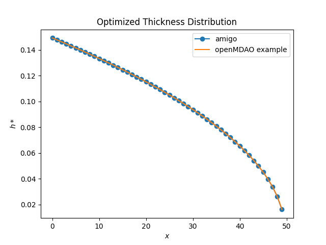
Here, you can see excellent agreement with OpenMDAO’s FEM formulation.

References

1. https://openmdao.org/newdocs/versions/latest/examples/beam_optimization_example.html