Derivative Free Optimization
There are many different derivative-free optimization (DFO) methods. Some are designed to be global optimizers: they seek the global minimum. However, other DFO methods only seek a local minimizer.
In this section, we’ll look at some heuristic methods, which include:
Genetic algorithms (or evolutionary algorithms) (GA or EA)
Particle swarm optimization (PSO)
We’ll also consider DFO algorithms that are not heuristic including:
Coordinate and pattern search methods
Model-based DFO
There are numerous papers in the literature with different heuristic optimization algorithms. Other methods in this class include:
Simulated annealing
Tabu search
Bee colony/ant colony/bacterial foraging, etc.
These methods can be useful since they can handle non-smooth functions, mixed-integer variables and categorical variables. Many people focus on the fact that these methods can find global solutions. But in my opinion, this is not surprising or a key selling point. This method also finds a global solution eventually:
Pick \(x_{0}\) and set \(f_{0} \leftarrow f(x_{0})\)
Pick \(x\) randomly
If \(f(x) < f_{0}\) Set \(x_{0} \leftarrow x\), \(f_{0} \leftarrow f(x)\)
Goto step 2
Terminology
Global convergence: Convergence to a local minimizer/critical point from any starting point - this is provable for many gradient-based methods.
Global optimizer: An optimizer which is designed to try to find the global minimum
Convergence: Does the optimization algorithm converge to a local or global optimum: Provable for many DFO methods, but this is the easy part
Rate of convergence: How quickly does the optimization algorithm converge when its near a local/global solution
We will look at some heuristic/metaheuristic optimization methods, but focus some attention on more-rigorous DFO methods:
Model-based DFO, good for smooth optimization
Pattern search, mesh-adaptive direct (MADS) search
We’ll look exclusively at derivative-free methods for optimization with bound constraints
\begin{equation*} \begin{aligned} \min_{x} \qquad & f(x) \\ \text{such that} \qquad & l \le x \le u \end{aligned} \end{equation*}
General constraints can be added by either:
Using penalty methods
Using augmented Lagrangian methods
Rejecting points that are infeasible (suitable for some types of algorithms)
Genetic Optimization Algorithms
Inspired by evolutionary processes in nature. These algorithms generally consist of a number of steps:
Initialization of the population
Selection
Crossover Reproduction/propagation of genetic traits
Mutation Injects a random variation into the population
Fitness evaluation
Replacement
These terms are in common usage.
The basic approach to genetic algorithms is as follows:
Create a set of samples in the design space, referred to as a population.
Apply some selection criteria to create a pool of design points to merge.
Apply a crossover operation to generate new data points, designed so that the newly generated samples are likely to retain good performing points.
Add randomness to the sample set.
The advantages of genetic algorithms are:
The variables are encoded so that they can easily accommodate continuous, integer and discrete design variables
The population can be distributed so that it tends not to get stuck in local minima
It can handle noisy functions or functions that are not smooth
It can be used for multi-objective optimization
The implementation is straightforward
The disadvantages of genetic algorithms are:
They can be expensive compared to gradient-based methods
Their computational cost scales strongly with the number of design variables
Genetic algorithms are better than brute force, but fundamentally rely on the stochastic mechanism to be classified as a global optimizer. Due to stochastic nature, performance of the GA must be measured using a statistically significant number of optimization runs.
Generic Genetic Algorithm Components
Encoding design points
Some GAs use real-valued design variables directly. However, many GAs use an encoding sequence to store the design variable values. In this approach, all the design variables become discrete.
We can represent a finite number of values using \(m\) bits. Real numbers between the lower value \(l\) and the upper value \(u\) can be found as follows:
\begin{equation*} x = l + (u - l)\left[ \sum_{i=0}^{n} b_{i} 2^{-k-1} \right] \end{equation*}
Here \(b\) is a binary vector such that \(b_{i} \in \{0, 1\}^{n}\). For instance, \(b = \begin{bmatrix} 0 & 1 & 1 & 0 & 1 \end{bmatrix}\).
Binary values can be encoded and decoded using the following functions:
def decode(b, low=0.0, high=1.0):
    val = 0.0
    for b0 in b[::-1]:
        val = 0.5 * (val + b0)
    return low + (high - low) * val
def encode(val, n=10, low=0.0, high=1.0):
    v = (val - low)/(high - low)
    b = []
    for i in range(n):
        if v >= 0.5:
            b.append(1)
            v = (v - 0.5)/0.5
        else:
            b.append(0)
            v = v/0.5
    return b
Note that there can be information loss
>>> decode(encode(0.5))
0.5
>>> decode(encode(0.65))
0.6494140625
>>> decode(encode(0.15))
0.1494140625
In practice, it’s better to use Gray code to encode the design variables. https://en.wikipedia.org/wiki/Gray_code.
Initialization
The goal of the initialization procedure is to obtain a sample set \(\{ x_{k} \}\) satisfying \(l \le x_{k} \le u\).
As a rule of thumb, the population should be 15 to 20 times the number of design variables. Often, the initial encoding sequence is \(b_{i}\) generated randomly
Selection
Determine a mating pool, by either:
Selecting the mates randomly
Select based on fitness: better members reproduce more than others the next population through a cross over operation
Mutation
Add randomness to the population
Particle Swarm Optimization
Particle Swarm Optimization (PSO) is a a stochastic, population-based optimization algorithm. Originally developed by J. Kennedy and R. Eberhart, a social-psychologist and an electrical engineer, respectively. The method is motivated by the idea of swarm intelligence. The authors defined swarm intelligence as
Swarm intelligence: Collective, intelligent behaviors emerge from a population of individuals interacting locally within their environment
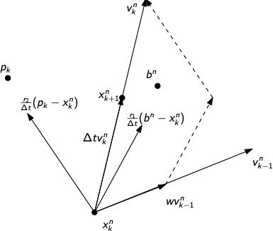
In PSO methods, a number of particles move in the design space. The particles are given dynamics that depend on:
An inertial effect
The best point achieved by the individual particle at any iteration
The best point achieved by any particle on the last iteration
For each particle \(n\):
\begin{equation*} \begin{aligned} x_{k+1}^{n} & = x_{k}^{n} + v_{k}^{n} \Delta t \\ v_{k}^{n} & = w v_{k-1}^{n} + \frac{r_{1}}{\Delta t} (b^{n} - x_{k}^{n}) + \frac{r_{2}}{\Delta t}(p_{k} - x_{k}^{n}) \end{aligned} \end{equation*}
Here the variables are defined such that
\(w\) is an inertial parameter
\(r_{1}\) is a random number on the interval \([0, c_{1}]\)
\(r_{2}\) is a random number on the interval \([0, c_{2}]\)
\(b^{n}\) is the best point for this particle, \(f(b^{n}) = \min_{k} f(x_{k}^{n})\)
\(p_{k}\) is the best point for this iteration, \(f(p_{k}) = \min_{n} f(x_{k}^{n})\)
The PSO algorithm can be defined as follows:
Select (possibly randomly) a set of particles \(\{x_{1}^{n}\}\), for \(n = 1,\ldots,N\)
Select randomly a set of particle velocities \(\{v_{1}^{n}\}\) for \(n = 1,\ldots,N\)
Set \(k = 1\)
Compute \(f(x_{k}^{n})\) for \(n = 1,\ldots,N\)
Update \(b^{n}\) and \(p_{k}\) using \(f(b^{n}) = \min_{k} f(x_{k}^{n})\) and \(f(p_{k}) = \min_{n} f(x_{k}^{n})\)
Update the velocities using:
\begin{equation*} v_{k}^{n} = w v_{k-1}^{n} + \frac{r_{1}}{\Delta t} (b^{n} - x_{k}^{n}) + \frac{r_{2}}{\Delta t}(p_{k} - x_{k}^{n}) \end{equation*}
Update the particle positions: \(x_{k+1}^{n} = x_{k}^{n} + v_{k}^{n}\)
Set \(k = k+1\) and go to step 4
Coordinate and pattern search methods
Coordinate search
At each iteration, search along a new coordinate direction \(e_{j}\) to approximately minimize \(f(x_{k} + \alpha e_{j})\)
The sequence in which we choose \(e_{j}\) is important
Any arbitrary selections of the sequence \(e_{j}\) will not necessarily converge
The steepest descent direction \(-\nabla f\) may become perpendicular to the coordinate search direction
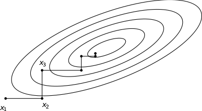
The sequence \(e_{1}, e_{2},\ldots,e_{n-1}, e_{n}, e_{n-1},\ldots, e_{2}, e_{1}, e_{2},\ldots\) can be shown to produce a convergent algorithm. Convergence can be slow, especially for functions not well-aligned with the coordinate axes.
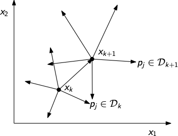
Pattern search methods
At each iteration perform a poll of all directions \(p_{j} \in \mathcal{D}_{k}\), where \(\mathcal{D}_{k}\) is a set of directions
Search directions must be carefully chosen so that we ensure that at least one direction \(p_{j} \in \mathcal{D}_{k}\) is a descent direction of \(f(x)\)
It turns out that we need at least \(n+1\) directions
We can recover coordinate search by selecting \(i\) and setting:
\begin{equation*} \mathcal{D}_{k} = \{e_{i}, -e_{i}\} \end{equation*}
However, this choice does not satisfy the property \(\kappa(\mathcal{D}) > 0\)
Another choice of \(\mathcal{D}\) are the coordinate directions:
\begin{equation*} \mathcal{D} = \{e_{1},e_{2},\ldots,e_{n},-e_1, -e_2,\ldots,-e_{n}\} \end{equation*}
Or the search directions:
\begin{equation*} p_{i} = \frac{1}{2n}e - e_{i}, \qquad i = 1,\ldots,n \qquad p_{n} = \frac{1}{2n} e \end{equation*}
Selecting the direction set \(\mathcal{D}_{k}\)
Consider the angle between the negative gradient direction and a direction \(p\):
\begin{equation*} \cos \theta = \frac{-\nabla f^{T}p}{||\nabla f|| \; ||p||} \end{equation*}
Since \(\nabla f\) may be any direction, we are interested in the worst case which can be written as:
\begin{equation*} \kappa(\mathcal{D}) = \min_{v} \max_{p \in \mathcal{D}} \frac{v^{T}p}{||v|| \; ||p||} \end{equation*}
We also must ensure that the length of the directions are bounded \(\beta_{\min} \le ||p|| \le \beta_{\max}\)
If the directions are bounded and \(\kappa(\mathcal{D}) > 0\), then at least one direction is a descent direction:
\begin{equation*} - \nabla f^{T}p \ge \kappa(\mathcal{D}) ||\nabla f|| \; ||p|| \ge \beta_{\min} \kappa(\mathcal{D}) ||\nabla f|| \end{equation*}
Pattern search algorithm
Select contraction/expansion parameters \(\theta\) and \(\phi\)
Select a convergence tolerance \(\gamma_{tol}\)
Pick \(x_{1}\) and an initial step length \(\gamma_{1} \ge \gamma_{tol}\) and an initial set of directions \(\mathcal{D}_{1}\)
Set \(k = 1\)
While \(\gamma_{k} > \gamma_{tol}\)
If \(f(x_{k} + \gamma_{k}p_{j}) < f(x_{k}) - \rho(\gamma_{k})\) for some \(p_{j} \in \mathcal{D}_{k}\)
Set \(x_{k+1} = x_{k} + \gamma_{k} p_{j}\)
Set \(\gamma_{k+1} = \phi \gamma_{k}\)
Else
Set \(x_{k+1} = x_{k}\)
Set \(\gamma_{k+1} = \theta \gamma_{k}\)
Set \(k = k + 1\) and go to step 5
\(\rho(t)\) is a function that satisfies \(\lim_{t \rightarrow 0} \frac{\rho(t)}{t} = 0\)
\(\rho(t) = \alpha t^{3/2}\) is a common choice
Model-based DFO
If the objective is smooth, we can approximate it using a quadratic model
This is similar to gradient-based methods that build quadratic models using gradient/Hessian information
At each iteration, we can form \(m_{k}(p)\) centered about the point \(x_{k}\) as follows:
\begin{equation*} m_{k}(p) = c + g^{T}p + \frac{1}{2}p^{T} B p \end{equation*}
However \(\nabla f\) is unavailable, so we have to interpolate
Assume that we can sample \(f(x)\) at the points \(\mathcal{Y} = \{y_{1},\ldots,y_{q}\}\) then \(m_{k}(\cdot)\) will satisfy the interpolation conditions:
\begin{equation*} m_{k}(y_{j} - x_{k}) = f(y_{j}), \qquad j = 1,\ldots,q \end{equation*}
We will need \(q = \frac{1}{2}(n + 1)(n+2)\) points to fully determine \(c\), \(g\) and \(B\)
Then we can use a trust-region framework and solve:
\begin{equation*} \min_{p} m_{k}(p) \qquad ||p|| \le \Delta_{k} \end{equation*}
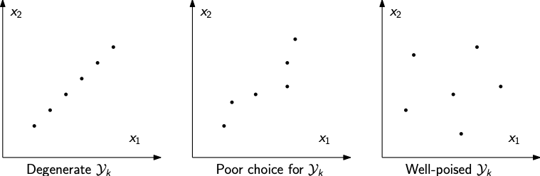
How we choose \(\mathcal{Y}_{k}\) is important - note that it is iteration-dependent
We cannot choose \(\mathcal{Y}_{k}\) arbitrarily - for instance if all the points in \(\mathcal{Y}_{k}\) lie on a line then we cannot perform interpolation
As the interpolation gets closer to a degeneracy like this, the poorer our interpolation will be
We can monitor how well-poised the interpolation set is by examining a shifted and scaled variant of the interpolation set \(\hat{\mathcal{Y}}\)
Once we have a full interpolation set, we may have to determine which \(y_{j} \in \mathcal{Y}_{k}\) to discard so that we only have \(q\) vectors
Improving the geometry of the interpolation set
Model-based DFO algorithms often implement a geometry-improvement step to ensure that \(\mathcal{Y}_{k}\) is well chosen
These algorithms remove a point \(y_{-} \in \mathcal{Y}_{k}\) and add a point \(y_{+}\) such that \(\mathcal{Y}_{k+1} = y_{+} \cup \left\{\mathcal{Y}_{k} \setminus y_{-} \right\}\)
These algorithms are often based on the Lagrange polynomials \(\ell_{i}(x; \mathcal{Y})\) for \(i = 1,\ldots,q\) defined such that:
\begin{equation*} \ell_{i}(y_{j}; \mathcal{Y}) = \delta_{ij} \end{equation*}
If we know the point we want to add, \(y_{+}\) we may choose to remove point \(y_{-} = y_{i_{\max}}\) chosen such that:
\begin{equation*} i_{\max} = \arg \max_{i} |\ell_{i}(y_{+}; \mathcal{Y}_{k})| \end{equation*}
In other words, remove the point corresponding to the Lagrange polynomial with the largest magnitude
Linear interpolation models
Consider first the case of linear interpolation with \(q = n+1\):
\begin{equation*} m_{k}(p) = f(x_{k}) + g^{T}p \end{equation*}
For the interpolant to match at the points \(y_{j}\) we must have:
\begin{equation*} f(x_{k}) + g^{T}(y_{j} - x_{k}) = f(y_{j}) \qquad \implies \qquad f(y_{j}) - f(x_{k}) = (y_{j} - x_{k})^{T}g \end{equation*}
Quadratic interpolation models
A quadratic model can be defined as follows:
\begin{equation*} m_{k}(p) = f(x_{k}) + g^{T}p + \frac{1}{2} p^{T} B p \end{equation*}
This leads to the interpolation conditions:
\begin{equation*} f(y_{j}) = f(x_{k}) + g^{T}(y_{j} - x_{k}) + \frac{1}{2} (y_{j} - x_{k})^{T} B (y_{j} - x_{k}) \end{equation*}
Writing \(s_{j} = y_{j} - x_{k}\), we can rewrite this condition as:
\begin{equation*} f(y_{j}) = f(x_{k}) + g^{T}s_{j} + \frac{1}{2} s_{j}^{T} B s_{j} \end{equation*}
We can write this as a linear system if we introduce the following notation for converting a matrix into a vector: \(\text{vec}(A) = a \in \mathbb{R}^{n(+1)/2}\)
\begin{equation*} \text{vec}(A)_{i + j(j-1)/2} = \left\{ \begin{array}{ll} \sqrt{2} A_{ij} \qquad & i \ne j \\ A_{ii} \qquad & i = j \end{array} \right. \end{equation*}
\begin{equation*} \text{vec}\begin{bmatrix} a_{11} & a_{12} & a_{13} \\ a_{12} & a_{22} & a_{23} \\ a_{13} & a_{23} & a_{33} \end{bmatrix} = \begin{bmatrix} a_{11} & \sqrt{2} a_{12} & a_{22} & \sqrt{2} a_{13} & \sqrt{2} a_{23} & a_{33} \end{bmatrix}^{T} \end{equation*}
Using this notation we can find the following:
\begin{equation*} s_{j}^{T} g + \frac{1}{2} \left[ \text{vec}(s_{j} s_{j}^{T})\right]^{T} \text{vec}(B) = f(x_{k}) - f(y_{j}) \end{equation*}
Minimum change update model
If we use a full quadratic model with interpolation we need to evaluate \((n+1)(n+2)/2\) points before we start optimization
This can be costly when \(n\) is large
Idea: Form an approximate quadratic model from \(\mathcal{O}(n)\) points and take up the additional degrees of freedom using least-Frobenius norm updates
In practice, we can use \(q = 2n +1\) points
This idea is similar to the BFGS/quasi-Newton updating schemes
Given model the \(m_{k}(p) = c_{k} + p^{T}g_{k} + \frac{1}{2} p^{T}B_{k} p\) we want to find the update to \(c_{k+1}\), \(g_{k+1}\) and \(B_{k+1}\) that solves the following minimum change problem:
\begin{equation*} \begin{aligned} \min_{c_{k+1}, g,_{k+1} B_{k+1}} \qquad & ||B_{k+1} - B_{k}||_{F} \\ \text{such that} \qquad & c_{k+1} + g_{k+1}^{T}(y_{j} - x_{k}) + \\ & \frac{1}{2} (y_{j} - x_{k})^{T}B_{k+1} (y_{j} - x_{k}) = f(y_{j}) \end{aligned} \end{equation*}
Setting \(s_{j} = y_{j} - x_{k}\) and defining \(c = c_{k+1} - c_{k}\), \(g = g_{k+1} - g_{k}\) and \(B = B_{k+1} - B_{k}\), we can define the problem:
\begin{equation*} \begin{aligned} \min_{c, g, B} \qquad & || B ||_{F} \\ \text{such that} \qquad & c + g^{T}s_{j} + \frac{1}{2}s_{j}^{T} B s_{j} = d_{j} = f(y_{j}) - m_{k}(y_{j} - x_{k}) \end{aligned} \end{equation*}
The Lagrangian for this problem can be written as follows:
\begin{equation*} \mathcal{L}(c, g, B) = \frac{1}{4} \sum_{ij} B_{ij}^2 - \sum_{j=1}^{q} \lambda_{j}\left( c + g^{T}s_{j} + \frac{1}{2} s_{j}^{T}B s_{j} - d_{j} \right) \end{equation*}
Differentiating with respect to \(c\), \(g\), and \(B\), respectively yields:
\begin{equation*} \sum_{j=1}^{q} \lambda_{j} = 0 \qquad \sum_{j=1}^{q} \lambda_{j} s_{j} = 0 \qquad B = \sum_{j=1}^{q} \lambda_{j} s_{j} s_{j}^{T} \end{equation*}
We can substitute this back into the expression for the equality constraints
\begin{equation*} c + g^{T}s_{i} + \frac{1}{2} \sum_{j=1}^{q} \lambda_{j} (s_{i}^{T}s_{j})^2 = d_{i} \end{equation*}
Writing \(A_{ij} = \frac{1}{2} (s_{i}^{T}s_{j})^2\), \(A \in \mathbb{R}^{q\times q}\) and \(S = \left[ s_{1}, s_{2}, s_{3} \ldots \right] \in \mathbb{R}^{n \times q}\) we obtain the following linear system:
\begin{equation*} \begin{bmatrix} A & e & S^{T} \\ e^{T} & 0 & 0 \\ S & 0 & 0 \\ \end{bmatrix} \begin{bmatrix} \lambda \\ c \\ g \\ \end{bmatrix} = \begin{bmatrix} d \\ 0 \\ 0 \\ \end{bmatrix} \end{equation*}
The Lagrange polynomials
We can derive a type of Lagrange polynomial that take the form:
\begin{equation*} m_{k+1}(p) - m_{k}(p) = \sum_{j=0}^{q-1} d_{j} \ell_{j}(p) \end{equation*}
Recall \(d_j = f(y_{j}) - m_{k}(y_{j} - x_{k})\)
The coefficients of these polynomials can be found as follows:
\begin{equation*} \begin{bmatrix} A & e & S^{T} \\ e^{T} & 0 & 0 \\ S & 0 & 0 \\ \end{bmatrix} \begin{bmatrix} \Lambda \\ \eta \\ \Gamma \end{bmatrix} = \begin{bmatrix} I \\ 0 \\ 0 \\ \end{bmatrix} \end{equation*}
Finally, the Lagrange polynomials take the following form:
\begin{equation*} \ell_{i}(p) = \eta_{i} + \Gamma_{i}^{T}p + \sum_{j=1}^{q} \frac{1}{2} \Lambda_{ij}(s_{j}^{T} p)^2 \end{equation*}
Changing the base point \(x_{k}\)
After solving the optimization problem, we obtain the new model function:
\begin{equation*} m_{k+1}(p) = c_{k+1} + p^{T} g_{k+1} + \frac{1}{2}p^{T}B_{k+1} p \end{equation*}
Where \(c_{k+1} = c + c_{k}\), \(g_{k+1} = g + g_{k}\) and \(B_{k+1} = B + B_{k}\)f
Note that the model \(m_{k+1}\) is centered about \(x_{k+1}\)
After the trust region problem, we obtain the new point \(x_{k+1}\), which we may want to use as the model base point for future iterations, in which case we need to update the model again:
\begin{equation*} \begin{aligned} c & \leftarrow c + g^{T}(x_{k+1} - x_{k}) + \frac{1}{2} (x_{k+1} - x_{k})^{T} B (x_{k+1} - x_{k}) \\ g & \leftarrow g + B (x_{k+1} - x_{k}) \\ \end{aligned} \end{equation*}
DFO algorithm
Simple model-based DFO algorithm, but provably convergent
Given \(x_{1}\), compute the \(2n+1\) initial points \(y_{j} \in \mathcal{Y}_1\)}
Set \(y_{1} = x_{1}\), \(y_{2k} = x_{1} + \Delta e_{k}\), and \(y_{2k+1} = x_{1} - \Delta e_{k}\)
Evaluate \(f(y_{j})\) for all \(y_{j} \in \mathcal{Y}_{1}\) and compute \(c_{1}\), \(g_{1}\) and \(B_{1}\)
Convergence check: \(||g_{k}|| \le \epsilon_{tol}\) \emph{and} \(\Lambda_{\mathcal{Y}_{k}} \le \Lambda_{0}\), (apply model improvement)}
Compute \(x^{*} = \arg \min m_{k}(p) \;\; ||p|| \le \Delta_{k}\)
Compute \(\rho_{k}\) and apply the trust region update to get \(\Delta_{k+1}\)
Add \(x_{k+1}\) to the set \(\mathcal{Y}_{k+1} = x_{k+1} \cup \{ \mathcal{Y}_{k} \setminus y_{-}\}\)
If successful trust region step center the trust region about the new best point \(x_{k+1}\)
Else discard points \(y_{j}\), \(||y_{j} - y_{1}|| > \Delta_{k}\) and apply model improvement to achieve \(\Lambda_{\mathcal{Y}_{k+1}} \le \Lambda_{0}\)
Compute and apply the updates \(c\), \(g\) and \(B\)
Return to step 3
Model error and the Lagrange polynomials
There is a strong connection between model error and the Lagrange polynomials
We can write the model \(m(x)\) in terms of the Lagrange polynomials as follows:
\begin{equation*} m(x) = \sum_{i=1}^{q} \ell_{i}(x) f(y_{i}) \end{equation*}
For a straightforward bound, consider the case of quadratic interpolation when \(f(x)\) has third derivatives that are continuous and bounded such that \(|f'''| \le \beta\)
In the quadratic case, the interpolation error bound takes the following form
\begin{equation*} |f(x) - m(x)| \le \frac{\beta}{6} \sum_{i=1}^{q} |\ell_{i}(x)| \; ||x - y_{i}||^3 \le q \frac{\beta}{6} \Lambda \Delta^{3} \end{equation*}
Here \(\Lambda = \max_{i} \max_{x} |\ell_{i}(x)|\) and \(\Delta = \max_{i} ||y_{i} - y_{1}||\). Note that large values of \(\ell_{i}(x)\) lead to poor error estimates.
How can we pick new points for \(\mathcal{Y}\) that will improve the geometry of the interpolation set?
First, we need a way to measure for the quality of a set of interpolation points
In general, we can write a polynomial as:
\begin{equation*} m(x) = \sum_{j=1}^{q} \alpha_{j} \phi_{j}(x) \end{equation*}
We can determine \(\alpha_{j}\) using a full interpolation scheme by evaluating \(f(x)\) at \(y_{j} \in \mathcal{Y}\):
\begin{equation*} m(y_{j}) = \sum_{j=1}^{q} \alpha_{j} \phi_{j}(y_{j}) = f(y_{j}) \end{equation*}
We can write this as a \(q \times q\) system of linear equations for \(\alpha\):
\begin{equation*} M(\phi, \mathcal{Y}) \alpha = F(\mathcal{Y}) \end{equation*}
Example
Consider, \(n = 2\) and \(d = 2\)
Therefore \(q = \frac{1}{2}(n+1)(n+2)= 6\)
Consider the natural basis of polynomials:
\begin{equation*} \phi(x) = \left\{ 1, x_1, x_2, x_1^2, x_1 x_2, x_{2}^2\right\} \end{equation*}
\begin{equation*} M(\phi, \mathcal{Y}) = \begin{bmatrix} \phi_{1}(y_{1}) & \phi_{2}(y_{1}) & \phi_{3}(y_{1}) & \ldots & \phi_{6}(y_{1}) \\ \phi_{1}(y_{2}) & \phi_{2}(y_{2}) & \phi_{3}(y_{2}) & \ldots & \phi_{6}(y_{2}) \\ \vdots & \vdots & \vdots & \vdots & \vdots \\ \phi_{1}(y_{6}) & \phi_{2}(y_{6}) & \phi_{3}(y_{6}) & \ldots & \phi_{6}(y_{6}) \\ \end{bmatrix} \end{equation*}
Geometry improvement algorithms
In general, the condition number of \(M(\phi, \mathcal{Y})\) is not a good indicator of the quality of \(\mathcal{Y}\)
We can scale the basis functions \(\phi(x)\) to get arbitrarily poor condition numbers, without affecting the interpolation
The classical measure of poisedness is based on the Lagrange polynomials such that \(\ell_{i}(y_{j}) = \delta_{j}\) and the model can be written:
\begin{equation*} m(x) = \sum_{i=1}^{q} \ell_{i}(x) f(y_{i}) \end{equation*}
Note that this requires that \(M(\phi, \mathcal{Y})\) be invertible
For any \(x\) in the convex hull of \(\mathcal{Y}\), and the
\begin{equation*} |m(x) - f(x)| \le \frac{q}{(d+1)!}G\Lambda_{\mathcal{Y}} \Delta^{d+1} \end{equation*}
Where \(d\) is the degree of the polynomial, \(G\) is a bound on the \(d+1\) derivative of \(f(x)\) in \(x \in \mathcal{B}(\Delta)\)
\(\Lambda_{\mathcal{Y}}\)-poised
The constant \(\Lambda_{\mathcal{Y}}\) is defined as:
\begin{equation*} \Lambda_{\mathcal{Y}} = \max_{i} \max_{x \in \mathcal{B}(\Delta)} |\ell_{i}(x)| \end{equation*}
We will try and maintain good geometry of our points by bounding \(\Lambda_{\mathcal{Y}}\) by adjusting the points in \(\mathcal{Y}\)
We will refer to sets \(\mathcal{Y}\) that have bounded \(\Lambda_{\mathcal{Y}}\) as \(\Lambda_{\mathcal{Y}}\)-poised
Large values of \(\Lambda_{\mathcal{Y}}\) are bad and lead to nearly-dependent Lagrange polynomials
When \(q = (n +1)(n+2)/2\), we can write the Lagrange polynomials as the solution to the following system of equations:
\begin{equation*} M^{T}(\phi, \mathcal{Y}) \ell(x) = \phi(x) \end{equation*}
We can use this to establish a bound on \(||\ell(x)||_{\infty}\)
In practice it is easier to work with a shifted and scaled version of the set:
\begin{equation*} \hat{\mathcal{Y}} = \left\{ 0, \frac{y_2 - y_1}{\Delta}, \frac{y_3 - y_1}{\Delta},\ldots,\frac{y_q - y_1}{\Delta} \right\} \end{equation*}
Where \(\Delta = \max_{y_{j} \in \mathcal{Y}} ||y_{j} - y_{1}||\)
This leads to the equivalent system of equations:
\begin{equation*} \hat{M}^{T}(\phi, \hat{\mathcal{Y}}) \ell\left( x \right) = \phi \left(\frac{x - y_1}{\Delta}\right) \end{equation*}
Some model improvement algorithms work by bounding \(||\hat{M}^{-1}||\)
These algorithms look like QR factorization or LU factorization
The norm \(||\hat{M}^{-1}||\) and the condition number \(\kappa(\hat{M})\) are related since \(||\hat{M}||\) is bounded
Model improvement algorithm based on Lagrange polynomials
At certain points in the model-based DFO algorithm we will want to improve the quality of the interpolation set
We will use an algorithm based on the Lagrange polynomials
The algorithm requires an upper bound \(\Lambda_{0}\) and proceeds as follows:
Compute \(\Lambda_{\mathcal{Y}} = \max_{i} \max_{x \in \mathcal{B}} |\ell_{i}(x)|\)
If \(\Lambda_{\mathcal{Y}} \le \Lambda_{0}\), quit: we have a set of points poised for interpolation
Otherwise pick \(j\) such that \(\max_{x \in \mathcal{B}} |\ell_{j}(x)| > \Lambda_{0}\)
Compute \(y_{j}^{+} = \max_{x \in \mathcal{B}} |\ell_{j}(x)|\)
Update the set, removing the old point, \(\mathcal{Y} \leftarrow \{ \mathcal{Y} \setminus y_{j} \} \cup y_{j}^{+}\)
Repeat until \(\Lambda_{\mathcal{Y}} \le \Lambda_{0}\)
For computational efficiency, \(\Lambda_{\mathcal{Y}}\) may be computed using an estimate/bound instead of computing the exact value of \(\max_{i} \max_{x \in \mathcal{B}} |\ell_{i}(x)|\)
Step 3 may be replaced with a simple heuristic such as simply selecting the point furthest from the center of the trust region
Criticality check:
Basic idea: Before checking \(|| g_{k} || \le \epsilon\), ensure \(\Lambda_{\mathcal{Y}} \le \Lambda_{0}\)
This will guarantee that the derivative approximate is bounded by the true derivative (otherwise \(\Lambda_{\mathcal{Y}}\) could be arbitrarily large)
Only quit once \(|| g_{k} || \le \epsilon\) and \(\Lambda_{\mathcal{Y}} \le \Lambda_{0}\)
Model improvement step:
Improve the model if the point did not change during the trust region step
The failure could be due to modeling inaccuracies as a result of a sample set that is not well-poised for interpolation
Various model-improvement algorithms exist, but all essentially solve an optimization problem to obtain new sample points
Wedge algorithms implement an approach to prevent poor sample point selection by modifying the trust region problem
[1]:
import numpy as np
import scipy.linalg as linalg
import matplotlib.pyplot as plt
class DFOpt:
def __init__(self, n, objfunc, A=None, b=None, lb=None, ub=None):
"""
Initialize the data for the derivative-free optimizer
"""
# Store the number of design variables in the problem
self.n = n
# Set the objective function pointer
self.objfunc = objfunc
# Compute the max number of interpolation points
self.m = 2*n + 1
# The trust region radius
self.tr = 1.0
self.tr_max = 2.0
self.eta = 0.25
self.max_lambda = 100.0
self.abs_opt_tol = 1e-3
# Set up the equality constraints
if A is not None and b is not None:
self.b = np.array(b)
self.A = np.array(A)
self.multipliers = np.zeros(len(self.b))
self.penalty = 20.0
else:
self.b = None
self.A = None
self.multipliers = None
self.penalty = 0.0
# Set which version of the trust region constraint to use
self.use_infty_tr = False
if lb is not None and ub is not None:
self.use_infty_tr = True
self.lb = np.array(lb)
self.ub = np.array(ub)
# Flag to determine whether to use the model improvement
# algorithm after failure of the trust region method
self.use_model_improvement = True
# Keep track of the number of function evaluations
self.fevals = 0
# The maximum number of iterations
self.max_major_iterations = 2000
# Draw the trust region on each iteration - should only
# be used for 2D problems and when debugging
self.plot_trust_region_iteration = False
# Set up the interpolation points
self.Y = np.zeros((self.n, self.m))
self.S = np.zeros((self.n, self.m))
# The vector of function values
self.fy = np.zeros(self.m)
# The W matrix and the right-hand-side
self.d = np.zeros(self.m + self.n + 1)
self.W = np.zeros((self.m + self.n + 1,
self.m + self.n + 1))
# The quadratic model coefficients
self.B = np.zeros((self.n, self.n))
self.g = np.zeros(self.n)
self.c = 0.0
return
def init_model(self, x0, delta):
"""
Initialize the model parameters at the starting point.
This uses a finite-difference stencil about the initial point
to create initial gradient and Hessian information.
Delta is a parameter which should be not too big but not too
small - i.e. don't think of it as a finite-difference
interval.
"""
# Evaluate the objective at f(x0)
self.Y[:, 0] = x0
self.fy[0] = self.objfunc(self.Y[:, 0])
for j in range(self.n):
# Evaluate the objective at f(x0 + delta*ej)
self.Y[:, 2*j+1] = x0
self.Y[j, 2*j+1] += delta
self.fy[2*j+1] = self.objfunc(self.Y[:, 2*j+1])
# Evaluate the objective at f(x0 - delta*ej)
self.Y[:, 2*(j+1)] = x0
self.Y[j, 2*(j+1)] -= delta
self.fy[2*(j+1)] = self.objfunc(self.Y[:, 2*(j+1)])
# Compute an approximate model about the initial point
self.c = self.fy[0]
for j in range(self.n):
self.g[j] = (self.fy[2*j+1] - self.fy[2*(j+1)])/delta
self.B[j, j] = (self.fy[2*j+1] - 2*self.fy[0] +
self.fy[2*(j+1)])/delta**2
# Add up the number of function evaluations
self.fevals += 2*self.n + 1
return
def update_model(self):
"""
Given the new point, compute the least-Frobenius norm update
"""
# Compute the new components of thee matrix since
# the points in Y may have changed order
for j in range(self.m):
self.S[:, j] = self.Y[:, j] - self.Y[:, 0]
# Compute S^{T}*S
A = 0.5*(np.dot(self.S.T, self.S))**2
# Set the components of the W matrix
self.W[:] = 0.0
self.W[:self.m, :self.m] = A
# Evaluate the inner product sj^{T}*B*sj for j = 1,...,m
sbs = np.zeros(self.m)
for j in range(self.m):
sbs[j] = np.dot(self.S[:, j], np.dot(self.B, self.S[:, j]))
# Compute dj = f(yj) - mk(yj)
self.d[:self.m] = (self.fy -
(self.c + np.dot(self.S.T, self.g) + 0.5*sbs))
# Set the unity components
self.W[self.m, :self.m] = 1.0
self.W[:self.m, self.m] = 1.0
# Set the S components
self.W[:self.m, self.m+1:] = self.S.T
self.W[self.m+1:, :self.m] = self.S
# Solve for the update
coef = linalg.solve(self.W, self.d)
# Apply the update to the quadratic model
self.c += coef[self.m]
self.g += coef[self.m+1:]
for j in range(self.m):
self.B += coef[j]*np.outer(self.S[:, j],
self.S[:, j])
return
def trust_region_l2(self, g, B, tr, max_iterations=10,
tol=1e-6):
"""
Solve (exactly) the possibly indefinite problem of minimizing
the function over the domain of interest
"""
# Compute the eigenvalues of the matrix B
lamb, Q = linalg.eigh(B)
# Compute the least value of h allowed
h = max(-lamb[0], 0.0) + 1e-3
# Now, iterate until convergence using Newton's method
for i in range(max_iterations):
A = B + h*np.eye(B.shape[0])
# Compute the cholesky factorization
try:
U = linalg.cholesky(A)
except:
U = linalg.cholesky(A)
# Compute U^{T}*U*p = -g
p = linalg.solve_triangular(U, g, trans='T')
p = -linalg.solve_triangular(U, p, trans='N')
# Compute the norm of the matrices
pnrm = linalg.norm(p)
if np.fabs((pnrm - tr)/tr) <= tol:
return p
# Compute U^{T}*q = p
q = linalg.solve_triangular(U, p, trans='T')
qnrm = linalg.norm(q)
# Print the trust region step
if pnrm == 0.0:
return p
dh = ((pnrm - tr)/tr)*(pnrm/qnrm)**2
if dh > 0.0:
h += dh
else:
return p
return p
def trust_region_linfty(self, g, B, lb, ub):
"""
Approximately solve the quadratic trust-region sub-problem
using a gradient projection method.
This method utilizes the piecewise linear path:
. { lb if x - t*g =< lb
xp(x - t*g, lb, ub) = { x - t*g if x - t*g in [lb, ub]
. { ub if x - t*g >= ub
The computation proceeds in three steps:
1. Determine the generalized Cauchy point using the gradient
projection method along the steepest descent path
2. Use the active set of constraints and solve approximately
the trust region problem
3. Project the final point back into the feasible region
"""
# Determine the break-point values
t = np.zeros(self.n)
for i in range(self.n):
if g[i] < 0.0:
t[i] = -ub[i]/g[i]
elif g[i] > 0.0:
t[i] = -lb[i]/g[i]
else:
t[i] = 1e20
# Sort the breakpoints
tsorted = np.sort(t)
# Initialize the x/p arrays
x = np.zeros(self.n)
p = -np.array(g)
t0 = 0.0
for k in range(self.n):
# Update the direction p
for i in range(self.n):
if t[i] <= t0:
p[i] = 0.0
# Determine the direction along which we're headed
f1 = np.dot(g, p) + np.dot(x, np.dot(B, p))
f2 = np.dot(p, np.dot(B, p))
# Determine what we should do:
if f1 > 0.0 or f2 == 0.0:
# The slope is increasing along this segment
break
dt = -f1/f2
if t0 + dt <= tsorted[k]:
x += dt*p
break
else:
x += (tsorted[k] - t0)*p
t0 = tsorted[k]
# # Compute the reduced Hessian matrix
# Z = np.eye(self.n)[:, inactive]
# # Compute the reduced Hessian
# Br = np.dot(Z.T, np.dot(B, Z))
# # Solve for the inactive gradient components
# x[inactive] = -linalg.solve(Br, g[inactive])
# # Move the solution back onto its bounds if they are violated
# for i in range(self.n):
# x[i] = max(x[i], lb[i])
# x[i] = min(x[i], ub[i])
return x
def discard_far_points(self, discard=1.5,
tr=1.0, max_lambda=10.0):
"""
Try to improve the Lambda-poised constant by discarding points
that are far from the center of the current interpolation.
This algorithm discards points that are further away than
'discard' and computes new points by maximizing the absolute
value of the associated Lagrange polynomial.
if ||yj - y1|| >= discard:
. yj^{+} = max_{||x - y1|| < tr} |lj(x)|
. Y = {Y \ yj} U yj^{+}
Here lj(x) is the corresponding Lagrange polynomial.
input:
discard: the discard radius
tr: the trust region radius
max_lambda: the maximum allowable lambda-poised constant
"""
while True:
# Compute the point that is the furthest away from
# the center point y1 = Y[:, 0]
jdis = 0
max_dist = 0.0
for j in range(1, self.m):
dist = linalg.norm(self.Y[:, j] - self.Y[:, 0])
if dist > max_dist:
jdis = j
max_dist = dist
# If the maximum distancce is less than the discard
# distance, then quit
if max_dist < discard:
return
# Now, compute the new Lagrange function within the new
# radius
rhs = np.zeros(self.m + self.n + 1)
rhs[jdis] = 1.0
coef = linalg.solve(self.W, rhs)
# Compute the specific Lagrange function
cj = coef[self.m]
gj = coef[self.m+1:]
# Compute the second order term for the Lagrange polynomial
Bj = np.zeros((self.n, self.n))
for n in range(self.m):
Bj += coef[n]*np.outer(self.S[:, n],
self.S[:, n])
# Maximize the lagrange polynomial
ppos = self.trust_region_l2(gj, Bj, tr)
lpos = np.fabs(cj + np.dot(gj, ppos) +
0.5*np.dot(ppos, np.dot(Bj, ppos)))
# Minimize the lagrange polynomial
pneg = self.trust_region_l2(-gj, -Bj, tr)
lneg = np.fabs(cj + np.dot(gj, pneg) +
0.5*np.dot(pneg, np.dot(Bj, pneg)))
# Select which point to discard
if lpos >= lneg:
self.Y[:, jdis] = self.Y[:, 0] + ppos
else:
self.Y[:, jdis] = self.Y[:, 0] + pneg
# Evaluate the objective at the new point
self.fy[jdis] = self.objfunc(self.Y[:, jdis])
self.fevals += 1
# Update the least-Frobenius norm model
self.update_model()
return
def compute_lambda_poised(self, tr=1.0, jstart=0):
"""
Compute the maximum absolute value of the Lagrange polyomials
within the given trust region and return the max value, the
index of the Lagrange polynomial and the location of the
maximum.
input:
tr: the trust region radius
output:
max_lagrange: the max absolute value of the Lagrange polyomial
jmax: the max index
ymax: the location of the max within the trust region
"""
jmax = 1
ymax = None
max_lagrange = 0.0
for j in range(jstart, self.m):
# Compute the components of the Lagrange polynomials
rhs = np.zeros(self.m + self.n + 1)
rhs[j] = 1.0
coef = linalg.solve(self.W, rhs)
# Compute the specific Lagrange function
cj = coef[self.m]
gj = coef[self.m+1:]
# Compute the coefficients
Bj = np.zeros((self.n, self.n))
for n in range(self.m):
Bj += coef[n]*np.outer(self.S[:, n],
self.S[:, n])
# Maximize the lagrange interpolant
ppos = self.trust_region_l2(gj, Bj, tr)
lpos = np.fabs(cj + np.dot(gj, ppos) +
0.5*np.dot(ppos, np.dot(Bj, ppos)))
# Minimize the lagrange interpolant
pneg = self.trust_region_l2(-gj, -Bj, tr)
lneg = np.fabs(cj + np.dot(gj, pneg) +
0.5*np.dot(pneg, np.dot(Bj, pneg)))
# Keep track of the maximum value seen thus far
if max(lpos, lneg) > max_lagrange:
max_lagrange = max(lpos, lneg)
jmax = j
if lpos >= lneg:
ymax = self.Y[:, 0] + ppos
else:
ymax = self.Y[:, 0] + pneg
return max_lagrange, jmax, ymax
def model_improvement(self, tr=1.0, max_lambda=10.0):
"""
Ensure that the set of interpolation points is well-poised for
interpolation over the trust region. This guarantees that our
model is fully linear/fully quadratic within the the trust
region given. This is the interpolation improvement algorithm
given by Conn et al. in an Introduction to Derivative Free
Optimization.
input:
tr: the trust region radius
max_lambda: the maximum allowable lambda-poised constant
"""
# Next, make sure that the Y-set is well-poised for
# interpolation
for i in range(self.m):
max_lagrange, jmax, ymax =\
self.compute_lambda_poised(tr=tr, jstart=1)
# Check if the maximum lambda-poised constant is exceeded
if max_lagrange > max_lambda:
fobj = self.objfunc(ymax)
self.fevals += 1
# If we're replacing the base point, then we have
# to re-adjust the least-Frobenius norm model
if jmax == 0:
# Calculate the displacement to the new point
p = ymax - self.Y[:, 0]
# Re-center the model about the new point
self.c += np.dot(self.g, p) + 0.5*np.dot(p, np.dot(self.B, p))
self.g[:] += np.dot(self.B, p)
# Set the new interpolation points
self.Y[:, jmax] = ymax
self.fy[jmax] = fobj
else:
return
# Update the model using the least-Frobenius norm
# update
self.update_model()
return
def plot_trust_region(self, x, ntr=2, n=75):
"""
Draw the original problem and the trust region problem.
Warning: This uses a lot of function evaluations and is
primarily intended for debugging/visualization.
"""
if plt is None:
return
xmin = self.Y[0, 0] - ntr*self.tr
xmax = self.Y[0, 0] + ntr*self.tr
ymin = self.Y[1, 0] - ntr*self.tr
ymax = self.Y[1, 0] + ntr*self.tr
# Create the range of x/y values to plot
x1 = np.linspace(xmin, xmax, n)
y1 = np.linspace(ymin, ymax, n)
R = np.zeros((n, n))
r = np.zeros((n, n))
# Create the contour plot for the real function
for j in range(n):
for i in range(n):
R[j, i] = self.objfunc([x1[i], y1[j]])
# Set the levels for the real function
Rlevels = np.min(R) + np.linspace(0, 1.0, 25)**2*(np.max(R) - np.min(R))
# Create the contours for the trust region subproblem
for j in range(n):
for i in range(n):
p = np.array([x1[i] - self.Y[0, 0],
y1[j] - self.Y[1, 0]])
r[j, i] = (self.c + np.dot(self.g, p) +
0.5*np.dot(p, np.dot(self.B, p)))
# Create the plot
fig = plt.figure(facecolor='w')
plt.contour(x1, y1, r, Rlevels)
plt.contour(x1, y1, R, Rlevels)
# Plot the interpolation points
for j in range(1, self.m):
plt.plot([self.Y[0, 0], self.Y[0, j]],
[self.Y[1, 0], self.Y[1, j]],
'-go', label=None)
# Plot the new point itself
plt.plot(x[0], x[1], 'ro')
# Plot the trust region
if self.use_infty_tr:
x0 = self.Y[0, 0]
y0 = self.Y[1, 0]
xt = [x0 - self.tr, x0 + self.tr, x0 + self.tr,
x0 - self.tr, x0 - self.tr]
yt = [y0 - self.tr, y0 - self.tr, y0 + self.tr,
y0 + self.tr, y0 - self.tr]
for i in range(5):
if xt[i] < self.lb[0]:
xt[i] = self.lb[0]
elif xt[i] > self.ub[0]:
xt[i] = self.ub[0]
if yt[i] < self.lb[1]:
yt[i] = self.lb[1]
elif yt[i] > self.ub[1]:
yt[i] = self.ub[1]
plt.plot(xt, yt, '-r', linewidth=2)
else:
cs = np.cos(np.linspace(0, 2*np.pi, 100))
ss = np.sin(np.linspace(0, 2*np.pi, 100))
plt.plot(self.Y[0, 0] + self.tr*cs,
self.Y[1, 0] + self.tr*ss, '-r', linewidth=2)
# Set the axis to be centered around the interpolation points
plt.axis([xmin, xmax, ymin, ymax])
plt.show()
return
def optimize(self, x, delta=0.1):
"""
Perform the derivative-free optimization.
This algorithm, as described above, uses a least-Frobenius
norm updating scheme to construct a quadratic model of the
objective function at each iteration. A simple gradient
criteria is used in conjunction with a test to ensure that the
interpolation is sufficiently accurate. This test is
implemented as a check on the maximum absolute value of the
Lagrange polynomial within the trust region.
"""
# Ensure that the design point is a numpy array
x = np.array(x)
# Initialize the quadratic model about the given point
self.init_model(x, delta)
# Update the model
self.update_model()
max_lagrange = 1.0
for k in range(self.max_major_iterations):
# Set the base point about which we'll construct the model
x0 = self.Y[:, 0]
# Add the term from the augmented Lagrangian (if needed)
if self.A is not None and self.b is not None:
con = np.dot(self.A, x0) - self.b
cval = self.penalty*con - self.multipliers
g = self.g + np.dot(self.A.T, cval)
else:
g = self.g
# If we have bound constraints, zero the gradient components
# associated with the bound constraints
gnrm = 0.0
if self.use_infty_tr:
for i in range(len(x0)):
if self.lb[i] < x0[i] and x0[i] < self.ub[i]:
gnrm += g[i]**2
gnrm = np.sqrt(gnrm)
else:
# Compute the gradient norm
gnrm = np.max(np.fabs(g))
# If the approximate gradient is zero, check if the model
# is good enough, then make a decision about exiting -
# without this check we could exit with bad gradient
# information
if gnrm < self.abs_opt_tol:
con_flag = True
if self.A is not None and self.b is not None:
con = np.dot(self.A, x0) - self.b
if np.sqrt(np.dot(con, con)) > self.abs_opt_tol:
self.multipliers -= self.penalty*con
else:
conf_flag = False
if con_flag:
max_lagrange, jmax, ymax =\
self.compute_lambda_poised(tr=self.tr)
# Check that the set is actually lambda poised
if max_lagrange < self.max_lambda:
break
else:
# Try the model improvement algorithm
self.model_improvement(tr=self.tr,
max_lambda=self.max_lambda)
# Recompute the gradient
if self.A is not None and self.b is not None:
con = np.dot(self.A, x0) - self.b
cval = self.penalty*con - self.multipliers
g = self.g + np.dot(self.A.T, cval)
else:
g = self.g
# Recompute the gradient and try the gradient
# test again
gnrm = 0.0
if self.use_infty_tr:
for i in range(len(x0)):
if self.lb[i] < x0[i] and x0[i] < self.ub[i]:
gnrm += g[i]**2
gnrm = np.sqrt(gnrm)
else:
# Compute the gradient norm
gnrm = np.max(np.fabs(g))
# Check if the gradient has converged
if gnrm < self.abs_opt_tol:
break
# Compute the lambda-poised constant - this is just used
# for printing/monitoring purposes, so it could be removed
if k % self.n == 0:
max_lagrange, jmax, ymax =\
self.compute_lambda_poised(tr=self.tr)
if max_lagrange > self.max_lambda:
# Perform the model improvement steps if required
self.model_improvement(tr=self.tr,
max_lambda=self.max_lambda)
# Set the old value of the objective function
x0 = self.Y[:,0]
fobj_old = self.fy[0]
# Set up the model problem. If this is unconstrained, use only the
# least-Frobenius norm model of the objective function. Otherwise,
# add the augmented Lagrangian terms from the constraints.
if self.A is not None and self.b is not None:
# Compute the constraint violation
con = np.dot(self.A, x0) - self.b
cval = self.penalty*con - self.multipliers
# Add the terms from the augmented Lagrangian
fobj_old += 0.5*self.penalty*np.dot(con, con)
fobj_old -= np.dot(self.multipliers, con)
# Add the augmented Lagrangian terms to the gradient/hessian
g = self.g + np.dot(self.A.T, cval)
B = self.B + self.penalty*np.dot(self.A.T, self.A)
else:
g = self.g
B = self.B
# Compute the l2 trust region solution
if self.use_infty_tr:
lb = np.zeros(self.lb.shape)
ub = np.zeros(self.ub.shape)
for i in range(len(self.lb)):
lb[i] = -self.tr
ub[i] = self.tr
if x0[i] - self.tr <= self.lb[i]:
lb[i] = self.lb[i] - x0[i]
if x0[i] + self.tr >= self.ub[i]:
ub[i] = self.ub[i] - x0[i]
# Solve the l-infinity trust region problem to find
# the next step
p = self.trust_region_linfty(g, B, lb, ub)
else:
p = self.trust_region_l2(g, B, self.tr)
# Compute the new point
x = x0 + p
# Compute the model reduction
mreduce = -np.dot(g, p) - 0.5*np.dot(p, np.dot(B, p))
# Evaluate the objective at the new point
fval = self.objfunc(x)
self.fevals += 1
fobj = 1.0*fval
# Add the terms from the augmented Lagrangian
if self.A is not None and self.b is not None:
con = np.dot(self.A, x) - self.b
fobj += 0.5*self.penalty*np.dot(con, con)
fobj -= np.dot(self.multipliers, con)
# Compute the ratio of the actual reduction to the
# predicted reduction
rho = (fobj_old - fobj)/mreduce
if k % 10 == 0:
print('\n%4s %5s %15s %10s %10s %10s %10s %10s'%(
'iter', 'evals', 'fobj', 'rho', '|g|',
'dmodel', 'tr', 'max|l(x)|'))
# Print the result to the screen
print('%-4d %-5d %15.8e %10.3e %10.3e %10.3e %10.3e %10.3e'%(
k, self.fevals, min(fobj, fobj_old), rho,
gnrm, mreduce, self.tr, max_lagrange))
# Draw the trust region step if required
if self.plot_trust_region_iteration:
self.plot_trust_region(x)
# Update the trust region size
if rho < 0.25:
self.tr *= 0.25
elif rho > 0.75:
self.tr = min(self.tr_max, 2*self.tr)
# If this was a successful step, update and re-center
# about the new point
if rho > self.eta:
# Discard the point that is furthest from
# the new base point
jdis = 0
max_dist = 0.0
for j in range(self.m):
dist = linalg.norm(self.Y[:, j] - x)
if dist > max_dist:
max_dist = dist
jdis = j
# Compute the step between the new center and the old
# center - store this in the step p
p = x - self.Y[:, 0]
if jdis != 0:
# Copy the old center point to the discarded index
self.Y[:, jdis] = self.Y[:, 0]
self.fy[jdis] = self.fy[0]
# Copy the new point to the old center point
self.Y[:, 0] = x[:]
self.fy[0] = fval
# Re-center the model about the new point
self.c += (np.dot(self.g, p) +
0.5*np.dot(p, np.dot(self.B, p)))
self.g[:] += np.dot(self.B, p)
# Use the least-Frobenius norm update scheme
self.update_model()
else:
# First, add the point that we just computed that has
# been rejected by removing the point that is furthest
# away from the center point.
jdis = 0
max_dist = 0.0
for j in range(1, self.m):
dist = linalg.norm(self.Y[:, j] - self.Y[:, 0])
if dist > max_dist:
jdis = j
max_dist = dist
self.fy[jdis] = fval
self.Y[:, jdis] = x
# Update the least-Frobenius norm update
self.update_model()
# Note: We must discard the points outside of the
# trust region AND execute a model improvement
# algorithm to ensure that the interpolation set is
# poised for interpolation - otherwise we will just
# have a set that is poised, but not within the trust
# region.
# Discard points from the interpolation set that
# are too far away from the solution
r = 1.5
self.discard_far_points(discard=r*self.tr, tr=self.tr,
max_lambda=self.max_lambda)
if self.use_model_improvement:
# Perform the model improvement steps if required
self.model_improvement(tr=self.tr,
max_lambda=self.max_lambda)
return x
class Problem1:
def __init__(self):
self.x_hist = []
return
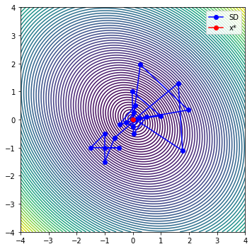
def obj_func(self, x):
self.x_hist.append(np.array(x))
return 2*x[0]**2 + 2*x[1]**2 + x[0]*x[1]
def gobj_func(self, x):
g = np.zeros(2)
g[0] = 4*x[0] + x[1]
g[1] = 4*x[1] + x[0]
return g
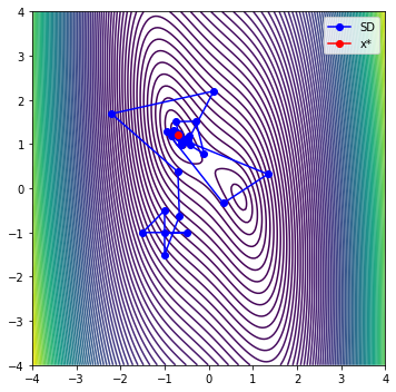
class Problem2:
def __init__(self):
self.x_hist = []
return
def obj_func(self, x):
self.x_hist.append(np.array(x))
return x[0]**4 + x[1]**2 + 2*x[0]*x[1] - x[0] - x[1]
def gobj_func(self, x):
g = np.zeros(2)
g[0] = 4*x[0]**3 + 2*x[1] - 1.0
g[1] = 2*x[1] + 2*x[0] - 1.0
return g
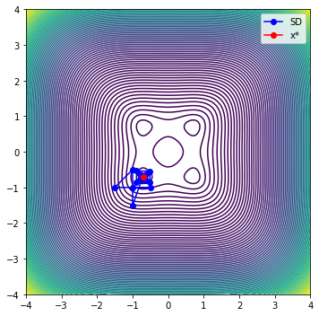
class Problem3:
def __init__(self):
self.x_hist = []
return
def obj_func(self, x):
self.x_hist.append(np.array(x))
return x[0]**4 + x[1]**4 + 1 - x[0]**2 - x[1]**2
def gobj_func(self, x):
g = np.zeros(2)
g[0] = 4*x[0]**3 - 2*x[0]
g[1] = 4*x[1]**3 - 2*x[1]
return g
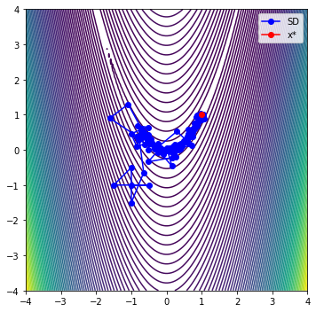
class Problem4:
def __init__(self):
self.x_hist = []
return
def obj_func(self, x):
self.x_hist.append(np.array(x))
return 100*(x[1]-x[0]**2)**2 + (1-x[0])**2
def gobj_func(self, x):
g = np.zeros(2)
g[0] = 200*(x[1]-x[0]**2)*(-2*x[0]) - 2*(1-x[0])
g[1] = 200*(x[1]-x[0]**2)
return g
class Problem5:
def __init__(self):
self.x_hist = []
return
def obj_func(self, x):
self.x_hist.append(np.array(x))
return -10*x[0]**2 + 10*x[1]**2 + 4*np.sin(x[0]*x[1]) - 2*x[0] + x[0]**4
def gobj_func(self, x):
g = np.zeros(2)
g[0] = -20*x[0] + 4*np.cos(x[0]*x[1])*x[1] - 2.0 + 4*x[0]**3
g[1] = 20*x[1] + 4*np.cos(x[0]*x[1])*x[0]
return g
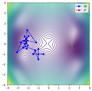
def plot_it_all(optimizer, problem, x_start=[-1.0, -1.0]):
"""
Plot a carpet plot with the search histories for steepest descent,
conjugate gradient and BFGS from the same starting point.
"""
# Create the data for the carpet plot
n = 150
xlow = -4.0
xhigh = 4.0
x1 = np.linspace(xlow, xhigh, n)
r = np.zeros((n, n))
for j in range(n):
for i in range(n):
r[j, i] = problem.obj_func([x1[i], x1[j]])
# Run steepest descent
x0 = np.array(x_start)
problem.x_hist = []
x = optimizer.optimize(x0, delta=0.5)
# print('|c(x)| ', np.sum(x) - 1.0)
# Assign the contour levels
levels = np.min(r) + np.linspace(0, 1.0, 75)**2*(np.max(r) - np.min(r))
# Copy out the steepest descent points
sd = np.zeros((2, len(problem.x_hist)))
for i in range(len(problem.x_hist)):
sd[0, i] = problem.x_hist[i][0]
sd[1, i] = problem.x_hist[i][1]
# Now, plot it all on a single plot
# Start plotting the figure
fig, ax = plt.subplots(1, 1, figsize=(5, 5))
ax.contour(x1, x1, r, levels)
plt.plot(sd[0, :], sd[1, :], '-bo', label='SD')
plt.plot(x[0], x[1], '-ro', label='x*')
ax.set_aspect('equal', 'box')
fig.tight_layout()
plt.legend()
plt.axis([xlow, xhigh, xlow, xhigh])
plt.show()
# x_start = np.random.uniform(low=-2.0, high=2.0, size=2)
x_start = [-1.0, -1.0]
# np.random.uniform(low=-2.0, high=2.0, size=2)
problems = [Problem1(), Problem2(),
Problem3(), Problem4(), Problem5()]
# problems = [Problem4()]
for problem in problems:
# Create the optimizer object
opt = DFOpt(2, problem.obj_func) #, A=[[1, 1]], b=[1])
opt.max_lambda = 10.0
opt.abs_opt_tol = 1e-3
opt.eta = 0.25
opt.tr = 0.5
opt.use_model_improvement = True
opt.plot_trust_region_iteration = False
# Plot all the functions
plot_it_all(opt, problem, x_start)
plt.show()
iter evals            fobj        rho        |g|     dmodel         tr  max|l(x)|
0    6      2.08946609e+00  9.588e-01  5.000e+00  3.036e+00  5.000e-01  1.000e+00
1    7      2.03143229e-02  9.066e-01  3.300e+00  2.282e+00  1.000e+00  1.000e+00
2    10     1.32808859e-03  1.194e+00  2.747e-01  1.591e-02  2.000e+00  2.986e+01
3    11     1.10861773e-03  1.663e+00  3.237e-02  1.319e-04  2.000e+00  2.986e+01
4    14     8.95141300e-06  8.801e-01  8.862e-02  1.249e-03  2.000e+00  5.483e+03
5    15     8.95141300e-06 -1.484e+00  9.541e-03  1.390e-05  2.000e+00  5.483e+03
6    20     1.23418650e-06  6.721e-01  9.432e-03  1.148e-05  5.000e-01  1.034e+00
7    21     2.91651770e-07  1.943e+00  1.754e-03  4.851e-07  5.000e-01  1.034e+00
8    24     2.91651770e-07 -3.014e+00  1.396e-03  2.643e-07  1.000e+00  8.227e+03
iter evals            fobj        rho        |g|     dmodel         tr  max|l(x)|
0    6      2.72130334e+00  8.869e-01  8.000e+00  3.697e+00  5.000e-01  1.000e+00
1    7      1.81945129e-01  8.569e-01  3.356e+00  2.963e+00  1.000e+00  1.000e+00
2    10    -4.04806453e-01  6.176e-01  1.917e+00  9.501e-01  2.000e+00  3.774e+01
3    11    -4.42528576e-01  2.298e+00  6.541e-01  1.642e-02  2.000e+00  3.774e+01
4    13    -4.42528576e-01 -1.095e-01  4.997e-01  3.200e+00  2.000e+00  1.065e+02
5    17    -4.42528576e-01 -5.409e-02  2.560e-01  2.631e-01  5.000e-01  1.065e+02
6    22    -4.89030270e-01  1.048e+00  5.896e-01  4.438e-02  1.250e-01  1.032e+00
7    23    -4.89030270e-01 -2.132e-01  2.906e-01  4.030e-02  2.500e-01  1.032e+00
8    27    -4.97919722e-01  9.562e-01  2.509e-01  9.297e-03  6.250e-02  4.609e+00
9    28    -4.99680749e-01  5.864e-01  7.024e-02  3.003e-03  1.250e-01  4.609e+00

iter evals            fobj        rho        |g|     dmodel         tr  max|l(x)|
10   30    -4.99820270e-01  2.031e-01  2.121e-02  6.869e-04  1.250e-01  5.590e+01
11   34    -4.99997926e-01  9.208e-01  4.277e-02  3.445e-04  3.125e-02  5.590e+01
12   36    -4.99999672e-01  7.105e-01  1.854e-03  2.458e-06  6.250e-02  2.500e+01
iter evals            fobj        rho        |g|     dmodel         tr  max|l(x)|
0    6      5.00209836e-01  5.831e-01  3.000e+00  8.571e-01  5.000e-01  1.000e+00
1    7      5.00209836e-01 -4.362e-01  9.759e-01  6.889e-02  5.000e-01  1.000e+00
2    11     5.00209836e-01 -1.161e-01  5.813e-02  8.091e-04  1.250e-01  1.284e+00
3    15     5.00010507e-01  1.064e+00  3.012e-02  1.873e-04  3.125e-02  1.284e+00
4    17     5.00009370e-01  6.041e+00  1.219e-03  1.882e-07  6.250e-02  8.613e+00
5    18     5.00006148e-01  2.602e+00  3.431e-03  1.239e-06  1.250e-01  8.613e+00
6    23     5.00006148e-01 -9.891e-01  5.734e-03  2.339e-03  2.500e-01  5.836e+04
7    27     5.00001867e-01  2.908e-01  1.063e-02  1.472e-05  6.250e-02  5.836e+04
8    29     5.00000810e-01  2.432e+00  3.137e-03  4.344e-07  6.250e-02  4.638e+01
9    30     5.00000810e-01 -1.398e+00  5.705e-03  5.896e-06  1.250e-01  4.638e+01
iter evals            fobj        rho        |g|     dmodel         tr  max|l(x)|
0    6      1.16164453e+02  8.336e-01  9.040e+02  3.453e+02  5.000e-01  1.000e+00
1    7      1.00111989e+01  5.254e-01  1.984e+02  2.021e+02  1.000e+00  1.000e+00
2    9      5.63252575e+00  7.679e-02  7.111e+01  5.702e+01  1.000e+00  1.355e+01
3    14     6.90248018e+00  1.593e-01  1.069e+02  1.951e+01  2.500e-01  1.355e+01
4    19     5.19131922e+00  1.007e+00  8.601e+01  4.788e+00  6.250e-02  1.035e+00
5    20     2.89362237e+00  1.155e+00  4.530e+01  1.989e+00  1.250e-01  1.035e+00
6    23     2.89362237e+00 -1.191e+00  4.464e+00  3.567e-01  2.500e-01  7.914e+01
7    28     2.71813578e+00  1.170e+00  8.467e+00  1.499e-01  6.250e-02  7.914e+01
8    30     2.47585312e+00  4.199e-01  2.409e+00  5.771e-01  1.250e-01  1.744e+01
9    31     2.21166464e+00  2.310e+00  2.498e+00  1.144e-01  1.250e-01  1.744e+01

iter evals            fobj        rho        |g|     dmodel         tr  max|l(x)|
10   33     2.21166464e+00 -2.286e-01  2.568e+01  1.965e+00  2.500e-01  4.465e+02
11   38     2.09729554e+00  3.011e-01  4.608e+00  3.799e-01  6.250e-02  4.465e+02
12   39     1.93818320e+00  6.510e-01  5.344e+00  2.444e-01  6.250e-02  4.125e+00
13   40     1.81045941e+00  1.058e+00  2.033e+00  1.207e-01  6.250e-02  4.125e+00
14   42     1.52517397e+00  7.834e-01  1.439e+00  3.641e-01  1.250e-01  2.849e+01
15   43     1.41220097e+00  6.427e+00  6.344e-01  1.758e-02  2.500e-01  2.849e+01
16   46     1.41220097e+00 -1.744e+00  2.214e+00  7.757e-02  5.000e-01  2.085e+02
17   49     1.40152229e+00  6.336e-02  2.332e+00  1.685e-01  1.250e-01  2.085e+02
18   54     1.34198127e+00  9.684e-01  2.384e+00  7.251e-02  3.125e-02  1.023e+00
19   55     1.20968482e+00  9.807e-01  2.099e+00  1.349e-01  6.250e-02  1.023e+00

iter evals            fobj        rho        |g|     dmodel         tr  max|l(x)|
20   58     1.05774483e+00  6.938e-01  1.935e+00  2.190e-01  1.250e-01  5.424e+01
21   59     8.49645113e-01  7.151e-01  5.995e+00  2.910e-01  1.250e-01  5.424e+01
22   61     7.56432698e-01  7.188e-01  3.652e-01  1.297e-01  1.250e-01  3.095e+01
23   62     6.72250096e-01  5.062e+00  6.263e-01  1.663e-02  1.250e-01  3.095e+01
24   65     6.72250096e-01 -7.389e+00  1.747e+00  3.010e-02  2.500e-01  1.558e+01
25   69     6.29750705e-01  2.328e+00  1.784e+00  1.826e-02  6.250e-02  1.558e+01
26   71     6.27159027e-01  1.143e+00  3.845e-01  2.268e-03  1.250e-01  1.503e+01
27   72     6.27036351e-01  1.558e+01  4.264e-02  7.874e-06  2.500e-01  1.503e+01
28   77     6.27036351e-01 -4.884e-01  1.107e+00  1.371e+00  5.000e-01  6.006e+04
29   82     6.27036351e-01 -3.985e-01  2.121e+00  1.351e-02  1.250e-01  6.006e+04

iter evals            fobj        rho        |g|     dmodel         tr  max|l(x)|
30   86     5.96213130e-01  7.785e-01  1.449e+00  3.959e-02  3.125e-02  3.649e+00
31   87     5.32604578e-01  1.741e+00  2.985e+00  3.654e-02  6.250e-02  3.649e+00
32   90     4.11747281e-01  1.777e+00  1.070e+00  6.800e-02  1.250e-01  1.902e+02
33   91     4.11747281e-01 -1.405e+00  2.611e+00  2.934e-01  2.500e-01  1.902e+02
34   95     3.48693180e-01  7.663e-01  2.631e+00  8.229e-02  6.250e-02  6.371e+00
35   96     2.66978979e-01  3.178e-01  2.810e+00  2.571e-01  1.250e-01  6.371e+00
36   98     2.41173344e-01  7.538e-02  7.134e-01  3.423e-01  1.250e-01  7.314e+01
37   103    2.21648058e-01  9.464e-01  3.835e+00  4.790e-02  3.125e-02  7.314e+01
38   105    2.08134595e-01  3.562e+00  6.012e-01  3.794e-03  6.250e-02  2.283e+01
39   106    1.40547618e-01  7.170e-01  7.865e-01  9.426e-02  1.250e-01  2.283e+01

iter evals            fobj        rho        |g|     dmodel         tr  max|l(x)|
40   108    1.40547618e-01 -8.676e-01  4.393e-01  8.576e-02  1.250e-01  7.049e+01
41   113    1.32167425e-01  2.011e+00  6.401e-01  4.167e-03  3.125e-02  7.049e+01
42   115    1.30981618e-01  1.124e+01  1.980e-01  1.055e-04  6.250e-02  1.760e+01
43   116    8.74425281e-02  4.449e-01  6.139e-01  9.785e-02  1.250e-01  1.760e+01
44   119    8.74425281e-02 -4.177e-01  3.249e-01  2.108e-02  1.250e-01  1.228e+03
45   124    7.31597240e-02  8.755e-01  1.982e+00  1.631e-02  3.125e-02  1.228e+03
46   126    5.57968784e-02  5.441e-01  7.150e-01  3.191e-02  6.250e-02  4.358e+01
47   127    4.58099455e-02  5.741e-01  2.602e-01  1.740e-02  6.250e-02  4.358e+01
48   128    4.58099455e-02 -1.149e+00  8.131e-02  2.875e-03  6.250e-02  3.062e+00
49   133    3.75286253e-02  5.856e-01  2.728e+00  1.414e-02  1.562e-02  3.062e+00

iter evals            fobj        rho        |g|     dmodel         tr  max|l(x)|
50   134    3.50750316e-02  3.457e+00  2.940e-01  7.098e-04  1.562e-02  4.268e+00
51   135    2.95047563e-02  7.456e-01  1.808e-01  7.471e-03  3.125e-02  4.268e+00
52   137    2.42686144e-02  4.641e-01  1.248e-01  1.128e-02  3.125e-02  3.105e+01
53   138    1.96557276e-02  1.723e+00  1.203e-01  2.677e-03  3.125e-02  3.105e+01
54   140    1.18707695e-02  1.019e+00  2.638e-01  7.642e-03  6.250e-02  1.177e+02
55   141    5.11772066e-03  6.729e-01  9.521e-02  1.004e-02  1.250e-01  1.177e+02
56   143    5.11772066e-03 -1.479e+01  3.113e+00  2.526e-04  1.250e-01  3.494e+03
57   147    2.69686754e-03  8.116e-01  1.925e+00  2.983e-03  3.125e-02  3.494e+03
58   149    2.69686754e-03 -6.816e-01  1.949e-01  2.306e-05  6.250e-02  8.325e+01
59   153    2.40863895e-03  9.748e-01  3.320e-01  2.957e-04  1.562e-02  8.325e+01

iter evals            fobj        rho        |g|     dmodel         tr  max|l(x)|
60   155    2.39492991e-03  5.448e+00  7.936e-03  2.516e-06  3.125e-02  3.541e+00
61   156    2.37155656e-03  2.194e+00  1.719e-02  1.065e-05  6.250e-02  3.541e+00
62   161    2.37155656e-03 -8.637e-01  4.043e-01  2.541e-02  1.250e-01  1.493e+05
63   165    2.37155656e-03 -7.389e-01  6.142e-01  1.332e-03  3.125e-02  1.493e+05
64   169    1.99009526e-03  4.642e-01  2.624e-01  8.217e-04  7.812e-03  1.038e+00
65   170    1.68019234e-03  3.935e-01  8.250e-02  7.876e-04  7.812e-03  1.038e+00
66   171    1.39872208e-03  9.810e-01  3.357e-02  2.869e-04  7.812e-03  3.358e+00
67   172    9.23318432e-04  9.891e-01  3.038e-02  4.806e-04  1.562e-02  3.358e+00
68   174    6.13842623e-04  2.100e-01  6.850e-02  1.474e-03  3.125e-02  1.082e+04
69   179    7.09733466e-04  1.039e+00  1.323e-01  2.055e-04  7.812e-03  1.082e+04

iter evals            fobj        rho        |g|     dmodel         tr  max|l(x)|
70   181    6.91689365e-04  4.481e+00  2.597e-02  4.027e-06  1.562e-02  4.132e+01
71   182    4.54761266e-04  2.309e+00  1.819e-02  1.026e-04  3.125e-02  4.132e+01
72   186    4.54761266e-04 -1.008e+00  1.287e-01  1.372e-03  6.250e-02  6.956e+03
73   189    1.98490890e-04  2.112e-01  5.137e-02  1.214e-03  1.562e-02  6.956e+03
74   194    3.76280516e-04  1.024e+00  1.053e-01  7.662e-05  3.906e-03  1.001e+00
75   195    2.51560082e-04  1.139e+00  1.943e-02  1.095e-04  7.812e-03  1.001e+00
76   198    2.16712516e-04  2.691e+00  1.259e-02  1.295e-05  1.562e-02  3.658e+02
77   199    3.43802065e-05  1.567e+00  6.313e-02  1.164e-04  3.125e-02  3.658e+02
78   203    3.43802065e-05 -1.895e-01  1.675e-02  1.942e-03  6.250e-02  2.858e+02
79   207    2.64978256e-06  1.891e-01  5.797e-02  1.678e-04  1.562e-02  2.858e+02

iter evals            fobj        rho        |g|     dmodel         tr  max|l(x)|
80   212    1.67557549e-05  8.369e-01  1.999e-02  2.106e-05  3.906e-03  1.011e+00
81   213    2.61697691e-06  1.550e+00  6.094e-03  9.122e-06  7.812e-03  1.011e+00
82   216    2.61697691e-06 -6.923e-01  1.235e-03  9.646e-06  1.562e-02  1.188e+02
83   220    8.54708326e-07  1.799e+00  1.303e-02  9.795e-07  3.906e-03  1.188e+02
84   222    8.54708326e-07 -5.683e+00  2.639e-03  5.331e-08  7.812e-03  7.959e+01
85   225    4.48309510e-09  4.231e-01  4.963e-03  2.010e-06  1.953e-03  7.959e+01
86   227    4.48309510e-09 -4.870e-01  2.163e-03  2.136e-07  1.953e-03  1.535e+01
87   230    4.08613134e-09  3.469e-02  2.252e-03  1.144e-08  4.883e-04  1.535e+01
88   235    3.31839623e-12  9.844e-01  2.123e-03  4.551e-09  1.221e-04  1.025e+00
<ipython-input-1-a10ff9ec3f1c>:153: LinAlgWarning: Ill-conditioned matrix (rcond=3.09692e-17): result may not be accurate.
  coef = linalg.solve(self.W, self.d)
<ipython-input-1-a10ff9ec3f1c>:337: LinAlgWarning: Ill-conditioned matrix (rcond=3.09692e-17): result may not be accurate.
  coef = linalg.solve(self.W, rhs)
<ipython-input-1-a10ff9ec3f1c>:153: LinAlgWarning: Ill-conditioned matrix (rcond=3.24362e-17): result may not be accurate.
  coef = linalg.solve(self.W, self.d)
<ipython-input-1-a10ff9ec3f1c>:337: LinAlgWarning: Ill-conditioned matrix (rcond=3.24362e-17): result may not be accurate.
  coef = linalg.solve(self.W, rhs)
<ipython-input-1-a10ff9ec3f1c>:153: LinAlgWarning: Ill-conditioned matrix (rcond=8.3527e-18): result may not be accurate.
  coef = linalg.solve(self.W, self.d)
<ipython-input-1-a10ff9ec3f1c>:337: LinAlgWarning: Ill-conditioned matrix (rcond=8.3527e-18): result may not be accurate.
  coef = linalg.solve(self.W, rhs)
<ipython-input-1-a10ff9ec3f1c>:153: LinAlgWarning: Ill-conditioned matrix (rcond=5.81836e-18): result may not be accurate.
  coef = linalg.solve(self.W, self.d)
<ipython-input-1-a10ff9ec3f1c>:397: LinAlgWarning: Ill-conditioned matrix (rcond=5.81836e-18): result may not be accurate.
  coef = linalg.solve(self.W, rhs)
<ipython-input-1-a10ff9ec3f1c>:153: LinAlgWarning: Ill-conditioned matrix (rcond=4.07157e-19): result may not be accurate.
  coef = linalg.solve(self.W, self.d)
<ipython-input-1-a10ff9ec3f1c>:397: LinAlgWarning: Ill-conditioned matrix (rcond=4.07157e-19): result may not be accurate.
  coef = linalg.solve(self.W, rhs)
<ipython-input-1-a10ff9ec3f1c>:153: LinAlgWarning: Ill-conditioned matrix (rcond=1.14153e-17): result may not be accurate.
  coef = linalg.solve(self.W, self.d)
<ipython-input-1-a10ff9ec3f1c>:397: LinAlgWarning: Ill-conditioned matrix (rcond=1.14153e-17): result may not be accurate.
  coef = linalg.solve(self.W, rhs)
iter evals            fobj        rho        |g|     dmodel         tr  max|l(x)|
0    6     -5.04141221e+00  1.009e+00  2.207e+01  1.131e+01  5.000e-01  1.000e+00
1    7     -1.76857425e+01  5.379e-01  1.613e+01  2.351e+01  1.000e+00  1.000e+00
2    9     -1.89238728e+01  1.496e-01  8.106e+00  8.278e+00  1.000e+00  1.299e+01
3    14    -2.05018448e+01  1.074e+00  1.280e+01  2.622e+00  2.500e-01  1.299e+01
4    16    -2.16441768e+01  3.598e-01  9.290e+00  3.175e+00  5.000e-01  1.164e+01
5    17    -2.21209982e+01  1.563e+00  3.784e+00  3.051e-01  5.000e-01  1.164e+01
6    20    -2.21209982e+01 -1.861e+00  6.594e-01  1.833e-01  1.000e+00  2.017e+01
7    24    -2.21429194e+01  1.024e+00  1.281e+00  2.140e-02  2.500e-01  2.017e+01
8    26    -2.21429194e+01 -1.435e+00  1.455e-02  2.746e-03  5.000e-01  1.243e+02
9    30    -2.21429194e+01 -6.537e-01  1.228e-01  2.913e-04  1.250e-01  1.243e+02

iter evals            fobj        rho        |g|     dmodel         tr  max|l(x)|
10   35    -2.21429575e+01  1.168e+00  4.572e-02  3.256e-05  3.125e-02  1.005e+00
11   36    -2.21429575e+01 -2.599e+00  4.389e-03  3.230e-07  6.250e-02  1.005e+00
12   41    -2.21429606e+01  8.832e-01  1.632e-02  3.535e-06  1.562e-02  1.003e+00
13   43    -2.21429606e+01 -5.189e-01  4.320e-03  2.516e-07  3.125e-02  2.195e+02
14   48    -2.21429606e+01  1.003e+00  1.099e-03  2.483e-08  7.812e-03  1.003e+00
15   50    -2.21429606e+01 -1.124e+00  1.277e-03  2.649e-08  1.562e-02  1.596e+03
[ ]: