Minimization of Quadratic Functions
A good first example is the minimization of quadratic functions. This will be useful in more general situations since we’ll often form a quadratic approximation of the objective function. We’ll study a quadratic function that takes the following form
\begin{equation*} f(x) = \frac{1}{2} x^{T} A x + b^{T} x + c, \end{equation*}
where \(x \in \mathbb{R}^{n}\), \(A = A^{T} \in \mathbb{R}^{n \times n}\). Since \(A\) is symmetric, it has an eigenvalue decomposition \(A = Q \Lambda Q^{T}\).
The gradient of \(f(x)\) is
\begin{equation*} \nabla f(x) = \frac{1}{2}(A x + A^{T} x) + b = A x + b \end{equation*}
The Hessian of \(f(x)\) is
\begin{equation*} H(x) = A \end{equation*}
To analyze \(f(x)\), it is convenient to use a change of basis to use an eigenvector basis as follows
\begin{equation*} x = Q \xi, \end{equation*}
where \(\xi \in \mathbb{R}^{n}\) are the components along each eigenvector. For each \(\xi\) point, we can recover the original point \(x = Q \xi\).
The advantage of this new basis is that it leads to a simplified form for the quadratic as follows
\begin{equation*} \begin{aligned} f(\xi) & = \frac{1}{2} \xi^{T} Q^{T} A Q \xi + \xi^{T} Q^{T} b + c = \frac{1}{2} \xi^{T} \Lambda \xi + \xi^{T} \bar{b} + c \\ &= \sum_{i=1}^{n} (\frac{1}{2}\lambda_{i} \xi_{i}^2 + \bar{b}_{i} \xi_{i} ) + c \end{aligned} \end{equation*}
where we have defined \(\bar{b} = Q^{T} b\) or component-wise \(\bar{b}_{i} = q_{i}^{T}b\). This is a separable function because it can be written as
\begin{equation*} f(\xi) = \sum_{i=1}^{n} f_{i}(\xi_{i}) \end{equation*}
so that we can minimize each \(f_{i}(\xi_{i})\) independently since each of these functions share no common variables. Focusing on a single function, \(f_{i}(\xi_{i})\) we have the form
\begin{equation*} f_{i}(\xi_{i}) = \frac{1}{2} \lambda_{i} \xi_{i}^{2} + \bar{b}_{i} \xi_{i} \end{equation*}
(We ignore the constant term because it has no impact on the location or characterization of the minimizer.)
Based on minimization of a one-dimensional function, we can make progress by considering a number of different cases. First, if \(\lambda_{i} = 0\) and \(\bar{b}_{i} = 0\), then the function is constant and any \(\xi_{i}\) we pick is a minimizer or maximizer! If \(\lambda_{i} = 0\) and \(\bar{b}_{i} \ne 0\), then the function is a line and there is no minimizer or maximizer.
Now, if \(\lambda_{i} \ne 0\), we have a quadratic function. Taking the derivative of \(f_{i}(\xi_{i})\) and set it equal to zero to obtain the critical point gives
\begin{equation*} \xi_{i}^{cr} = -\frac{\bar{b}_{i}}{\lambda_{i}} \end{equation*}
Finding the second derivative of \(f_{i}(\xi_{i})\) gives just \(\lambda_{i}\). So if \(\lambda_{i} \ne 0\), then when \(\lambda_{i} > 0\), we have a minimizer at \(\xi_{i}^{*} = - {\bar{b}_{i}}/{\lambda_{i}}\). Whereas if \(\lambda_{i} < 0\), we have a maximizer at \(\xi_{i} = {\bar{b}_{i}}/{\lambda_{i}}\).
As a result we have the following cases:
If \(\lambda_{i} > 0\), then \(\xi_{i}^{*}\) is a minimizer
If \(\lambda_{i} < 0\), then \(\xi_{i}^{*}\) is a maximizer
If \(\lambda_{i} = 0\) and \(\bar{b}_{i} = 0\), then any value of \(\xi_{i}\) is a minimizer or maximizer
If \(\lambda_{i} = 0\) and \(\bar{b}_{i} \ne 0\), then the function is unbounded from below (no minimizer)
We can now apply these conditions to all the eigenvalues.
If \(A\) is positive definite, then all \(\xi_{i}\) directions are minimizers
If \(A\) is positive semi-definite, then the function is either unbounded from below or has a non-unique minimizer depending on \(b\)
If \(A\) is indefinite, negative semi-definite or negative definite, then the function is unbounded from below and has no minimizer
For case 1, we have that the location of the minimizer is given by
\begin{equation*} \xi^{*} = -\Lambda^{-1}\bar{b} = -\Lambda^{-1} Q^{T} b \end{equation*}
Transforming this back into the design coordinates gives
\begin{equation*} x^{*} = Q \xi^{*} = -Q \Lambda^{-1} Q^{T} b = -A^{-1} b \end{equation*}
Note that \(x^{*} = -A^{-1} b\) is a minimizer only if \(A\) is positive definite!
For case 2, we have that \(\lambda_{i} \ge 0\). For those \(\lambda_{i} = 0\), we have to test the conditions on \(\bar{b}_{i} = q_{i}^{T} b\). So if \(q_{i}^{T} b = 0\) for each \(i\) where we have \(\lambda_{i} = 0\), then we have a non-unique minimizer, because we can move along \(\xi_{i}\) without changing the function value.
Note that for case 2, the matrix \(A\) is singular, so we have to be careful!
In the case where \(q_{i}^{T} b = 0\) for all \(\lambda_{i} = 0\), then minimizer can be expressed as follows:
\begin{equation*} \xi_{i}^{*} = \left\{ \begin{array}{lr} -\frac{\bar{b}_{i}}{\lambda_{i}} & \lambda_{i} \ne 0 \\ 0 & \lambda_{i} = 0 \\ \end{array} \right. \end{equation*}
Multiplying both sides by \(\lambda_{i}\), we see that \(\Lambda \xi^{*} = -\bar{b}\), but the matrix \(\Lambda\) has zeros at some entries along the diagonal. To address these, we add a matrix \(E\) whose entries are all zero, except on the diagonal we place a 1 wherever there was a zero eigenvalue. Note that in this case, \(\bar{b}_{i} = 0\), so we are setting \(\xi_{i}^{*} = 0\) whenever \(\lambda_{i} = 0\). Now we can write
\begin{equation*} \begin{aligned} (\Lambda + E) \xi^{*} &= -\bar{b} \\ (\Lambda + E) Q^{T} x^{*} &= -Q^{T} b \\ Q (\Lambda + E) Q^{T} x^{*} &= -b \\ (Q \Lambda Q^{T} + Q E Q^{T}) x^{*} &= -b \\ \left(A + \sum_{i s.t. \lambda_{i} = 0} q_{i} q_{i}^{T} \right) x^{*} &= -b \\ \bar{A} x^{*} &= -b \\ \end{aligned} \end{equation*}
where here we have define
\begin{equation*} \bar{A} = A + \sum_{i s.t. \lambda_{i} = 0} q_{i} q_{i}^{T} \end{equation*}
Note that \(\bar{A}\) is nonsingular.
In the following, we consider several examples that show several quadratic functions.
Examples
Example 1
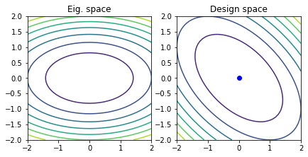
Consider the quadratic function
\begin{equation*} f(x) = x_{1}^2 + x_{2}^2 + x_{1} x_{2} \end{equation*}
The \(A\) matrix and \(b\) vector for this case are
\begin{equation*} A = \begin{bmatrix} 2 & 1 \\ 1 & 2 \\ \end{bmatrix} \quad\quad b = \begin{bmatrix} 0 \\ 0 \end{bmatrix} \end{equation*}
The eigenvalues for this case are \(\lambda_{1} = 1\), \(\lambda_{2} = 3\). Therefore, the minimizer is the point \(x^{*} = (0, 0)\).
Example 2
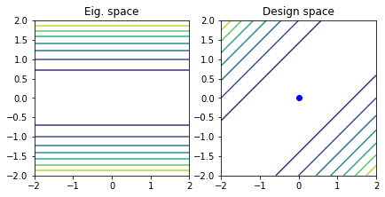
Consider the quadratic function
\begin{equation*} f(x) = \frac{1}{2} x_{1}^2 + \frac{1}{2} x_{2}^2 - x_{1} x_{2} \end{equation*}
The \(A\) matrix and \(b\) vector for this case are
\begin{equation*} A = \begin{bmatrix} 1 & -1 \\ -1 & 1 \\ \end{bmatrix} \quad\quad b = \begin{bmatrix} 0 \\ 0 \end{bmatrix} \end{equation*}
The eigenvalues of the matrix \(A\) are \(\lambda_{1} = 0\), \(\lambda_{2} = 2\). Therefore the matrix is positive semi-definite. Since \(b\) is zero, there is an infinite line of minimizers. The matrix of eigenvectors is
\begin{equation*} Q = \frac{1}{\sqrt{2}} \begin{bmatrix} 1 & 1 \\ 1 & -1 \end{bmatrix} \end{equation*}
The line of minimizers is given by
\begin{equation*} x^{*} = \alpha q_{1} = \dfrac{\alpha}{\sqrt{2}} \begin{bmatrix} 1 \\ 1 \end{bmatrix} \end{equation*}
where \(\alpha \in \mathbb{R}\) is arbitrary. Note that the non-singular matrix \(\bar{A}\) is
\begin{equation*} \bar{A} = A + q_{1} q_{1}^{T} = \begin{bmatrix} 1 & -1 \\ -1 & 1 \\ \end{bmatrix} + \frac{1}{2} \begin{bmatrix} 1 & 1 \\ 1 & 1 \end{bmatrix} = \frac{1}{2} \begin{bmatrix} 3 & -1 \\ -1 & 3 \end{bmatrix} \end{equation*}
Example 3
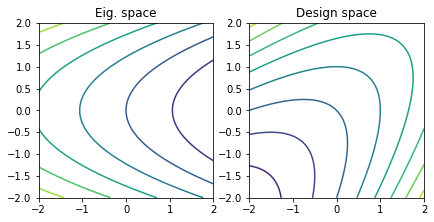
Consider the quadratic function
\begin{equation*} f(x) = \frac{1}{2} x_{1}^2 + \frac{1}{2} x_{2}^2 - x_{1} x_{2} + x_{1} + x_{2} \end{equation*}
The \(A\) matrix and \(b\) vector for this case are
\begin{equation*} A = \begin{bmatrix} 1 & -1 \\ -1 & 1 \\ \end{bmatrix} \quad\quad b = \begin{bmatrix} 1 \\ 1 \end{bmatrix} \end{equation*}
The \(A\) matrix is the same as Example 2. Since \(\lambda_{1} = 0\), and \(q_{1}^{T} b = \sqrt{2} \ne 0\), the function is unbounded from below. There is no minimizer.
Example 4
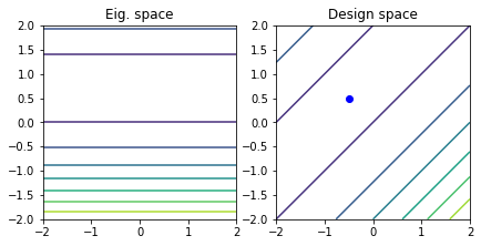
Consider the quadratic function
\begin{equation*} f(x) = \frac{1}{2} x_{1}^2 + \frac{1}{2} x_{2}^2 - x_{1} x_{2} + x_{1} - x_{2} \end{equation*}
The \(A\) matrix and \(b\) vector for this case are
\begin{equation*} A = \begin{bmatrix} 1 & -1 \\ -1 & 1 \\ \end{bmatrix} \quad\quad b = \begin{bmatrix} 1 \\ -1 \end{bmatrix} \end{equation*}
The \(A\) matrix is the same as Example 2. However, since \(\lambda_{1} = 0\) and \(q_{1}^{T} b = 0\), there are an infinite line of minimizers.
To find this line, we can first solve for a point along the line as
\begin{equation*} x^{*} = - \bar{A}^{-1} b = - 2 \begin{bmatrix} 3 & -1 \\ -1 & 3 \end{bmatrix}^{-1} \begin{bmatrix} 1 \\ -1 \end{bmatrix} = - \frac{1}{4} \begin{bmatrix} 3 & 1 \\ 1 & 3 \end{bmatrix} \begin{bmatrix} 1 \\ -1 \end{bmatrix} = \frac{1}{2} \begin{bmatrix} -1 \\ 1 \end{bmatrix} \end{equation*}
However, we can move along the direction \(q_{1}\) without changing the value of the quadratic. As a result, this is a line of minimizers
\begin{equation*} x^{*} = \frac{1}{2} \begin{bmatrix} -1 \\ 1 \end{bmatrix} + \dfrac{\alpha}{\sqrt{2}} \begin{bmatrix} 1 \\ 1 \end{bmatrix} \end{equation*}
Example 5
Consider the quadratic function
\begin{equation*} f(x) = 2 x_{1}^2 - 2 x_{2}^2 + x_{1} x_{2} \end{equation*}
The \(A\) matrix and \(b\) vector for this case are
\begin{equation*} A = \begin{bmatrix} 4 & 1 \\ 1 & -4 \\ \end{bmatrix} \quad\quad b = \begin{bmatrix} 0 \\ 0 \end{bmatrix} \end{equation*}
The eigenvalues can be obtained by solving
\begin{equation*} \det(A - \lambda 1) = -(4 - \lambda)(4 + \lambda) - 1 = \lambda^{2} - 17 = 0 \end{equation*}
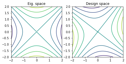
Therefore the eigenvalues are \(\lambda_{1} = -\sqrt{17}\) and \(\lambda_{2} = \sqrt{17}\). The matrix \(A\) is indefinite. Therefore the function \(f(x)\) is a saddle point and unbounded from below. There is no minimizer.
[4]:
import numpy as np
import matplotlib.pylab as plt

def quadratic_decomposition(A, b, tol=1e-6):
    # Perform the eigenvalue decomposition
    lam, Q = np.linalg.eigh(A)

    # Compute bar{b} = Q^{T}*b
    bbar = np.dot(Q.T, b)

    if lam[0] > tol:
        print('Positive definite; Unique minimizer')
        xstar = -np.linalg.solve(A, b)
    elif lam[0] > -tol:
        # The problem is semi-definite

        # Keep track of whether this problem is unbounded from below or not
        unbounded = False

        # Copy the values of A to a new matrix
        Abar = np.array(A, dtype=float)

        for index, eig in enumerate(lam):
            if np.fabs(eig) < tol:
                # Add the outer product of the two vectors to make the matrix
                # Abar non-singular
                Abar += np.outer(Q[:, index], Q[:, index])

                # Keep track of whether bbar is zero or not
                if np.fabs(bbar[index]) > tol:
                    unbounded = True

        if not unbounded:
            print('Semi-definite; Infinite number of minimizers')
            xstar = -np.linalg.solve(Abar, b)
        else:
            print('Semi-definite; Quadratic unbounded')
            xstar = None
    else:
        # The smallest eigenvalue is negative
        print('Indefinite; Quadratic unbounded')
        xstar = None

    if xstar is not None:
        print('xstar = ', xstar)

    if b.shape[0] == 2:
        m = 50
        x1 = np.linspace(-2, 2, m)
        x2 = np.linspace(-2, 2, m)
        X1, X2 = np.meshgrid(x1, x2)

        Fx = np.zeros(X1.shape)
        Fxi = np.zeros(X1.shape)

        for j in range(m):
            for i in range(m):
                x = np.array([X1[i,j], X2[i,j]])
                Fx[i, j] = 0.5*np.dot(x, np.dot(A, x)) + np.dot(b, x)
                Fxi[i, j] = 0.5*np.sum(lam*x**2) + np.dot(bbar, x)

        fig, ax = plt.subplots(1, 2)
        ax[0].contour(X1, X2, Fxi)
        ax[1].contour(X1, X2, Fx)
        if xstar is not None:
            ax[1].plot([xstar[0]], [xstar[1]], 'bo')
        ax[0].set_aspect('equal', 'box')
        ax[0].set_title('Eig. space')

        ax[1].set_aspect('equal', 'box')
        ax[1].set_title('Design space')
        fig.tight_layout()
        plt.show()

# Positive definite example
A = np.array([[2.0, 1.0], [1.0, 2.0]])
b = np.zeros(2)
quadratic_decomposition(A, b)

# Semi-definite examples
A = np.array([[1.0, -1.0], [-1.0, 1.0]])
b = np.zeros(2)
quadratic_decomposition(A, b)

b = np.array([1.0, 1.0])
quadratic_decomposition(A, b)

b = np.array([1.0, -1.0])
quadratic_decomposition(A, b)

# Negative definite examples
A = np.array([[4.0, 1.0], [1.0, -4.0]])
b = np.zeros(2)
quadratic_decomposition(A, b)
Positive definite; Unique minimizer
xstar =  [-0. -0.]
Semi-definite; Infinite number of minimizers
xstar =  [-0. -0.]
Semi-definite; Quadratic unbounded
Semi-definite; Infinite number of minimizers
xstar =  [-0.5  0.5]
Indefinite; Quadratic unbounded
[ ]: