2026 Class Project: Race Car Minimum Lap Time

Introduction

Lap time simulation of racing vehicles is nowadays widely used to predict car performance on race tracks and to optimize the vehicle setup before track tests. The two most common methods used to perform such simulations are the quasi-steady-state and the optimal control approaches. In the quasi-steady-state method, a fixed trajectory is provided as input data, the path is divided into small segments, and the vehicle maximum speed is calculated at each corner apex. Starting from these known points, acceleration and braking zones are reconstructed by forward and backward integration. Such simulations are fast to compute and very robust, which is why they remain the most widely used performance tools in racing teams. However, the fixed trajectory represents a fundamental limitation for the accuracy of the result, since the method cannot discover that a different line through a corner sequence might yield a faster overall lap.

The optimal control approach removes this limitation entirely. Rather than prescribing a trajectory, the racing line emerges as part of the solution. The optimizer determines simultaneously all driver inputs (steering, throttle, braking) and the resulting vehicle path, subject to the full nonlinear vehicle dynamics and all physical constraints. The trade-offs that a human driver must resolve by intuition and experience, such as how late to brake, how much to sacrifice corner entry speed for a better exit, or when to use the full width of the track, are handled automatically by the optimization. In practice, the continuous optimal control problem is transcribed into a large but finite nonlinear program (NLP) using direct collocation, and then solved numerically.

In this work, the minimum lap time problem (MLTP) is solved using a formulation inspired by the work of Christ et al. [1], originally developed at the Technical University of Munich for the Roborace autonomous racing competition. The vehicle is modeled as a planar rigid body with a double-track configuration in which all four wheels are treated independently. Lateral tire forces are computed with an extended Pacejka model that accounts for load-dependent friction degression, and wheel normal loads follow from a quasi-steady-state load transfer model that includes aerodynamic downforce. The track is described in curvilinear coordinates with arc length as the independent variable, so that time itself becomes the quantity to be minimized. Physical limits are enforced through Kamm’s friction circle at each wheel, engine power constraints, actuator rate bounds, and track boundary conditions. Because the track is a closed circuit, the solution must be periodic: the vehicle state at the end of the lap must match the state at the start. As shown in Figure 1, during cornering the heading velocity deviates from the vehicle’s longitudinal axis by the yaw angle \(\beta\), while the vehicle simultaneously rotates about its center of gravity at the yaw rate \(\omega_z\) and experiences lateral acceleration and aerodynamic drag. Accurately resolving these coupled effects is the central challenge addressed in this work.

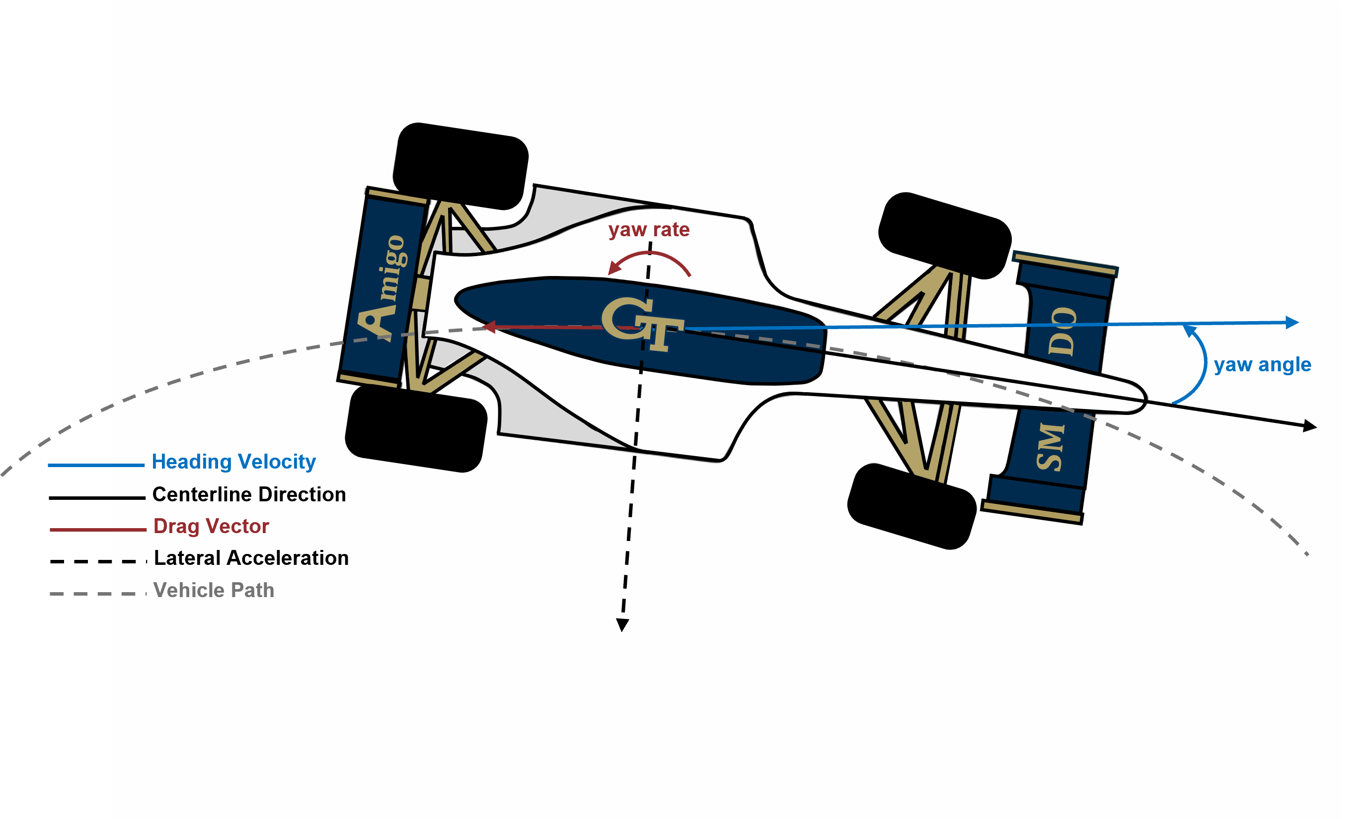
Figure 1. Diagram showing a race car attitude in cornering.

The remainder of this document presents the track model, the vehicle model, the optimal control problem formulation, and the numerical method.

Track Model

Curvilinear Coordinates

The track is described using a curvilinear coordinate system that uses the arc length \(s\) of a reference line (the track centerline) as the independent variable. This approach, widely used in the racing literature, offers several advantages: it provides a compact description of the vehicle’s progress along the circuit, simplifies the treatment of track boundary constraints, and naturally handles the periodicity of a closed lap.

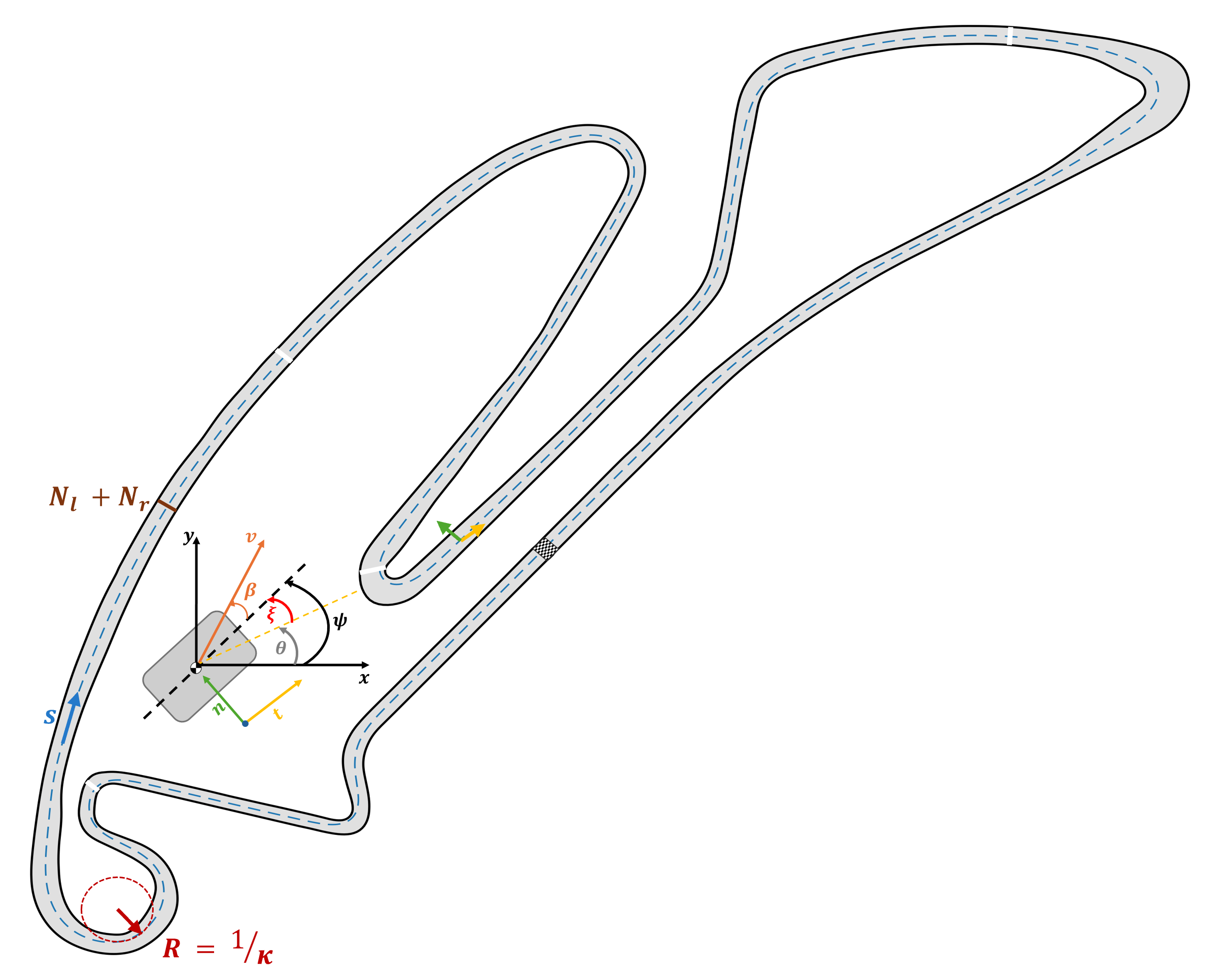
Figure 2. Curvilinear coordinate system on the Berlin Formula E circuit.

The vehicle position relative to the track is described by the lateral displacement \(n\) from the reference line (positive to the left) and the relative heading angle \(\xi\) between the vehicle’s longitudinal axis and the tangent to the reference line. At any point \(s\), the track geometry is characterized by the curvature \(\kappa(s)\), equal to the inverse of the local radius of curvature \(R(s)\), and the track half-widths \(N_l(s)\) and \(N_r(s)\) to the left and right of the centerline.

The time evolution of the curvilinear coordinates is:

\[\dot{s} = \frac{v \cos(\xi + \beta)}{1 - n\kappa}\]

\[\dot{n} = v \sin(\xi + \beta)\]

\[\dot{\xi} = \omega_z - \kappa \frac{v \cos(\xi + \beta)}{1 - n\kappa}\]

where \(v\) is the vehicle speed, \(\beta\) is the body sideslip angle, and \(\omega_z\) is the yaw rate.

Change of Independent Variable

In race line optimization, it is standard practice to use the path coordinate \(s\) as the independent variable rather than time \(t\). The time to be minimized therefore becomes a dependent variable. This choice eliminates \(s\) as a state variable, reducing the problem size. It also enables a simple description of track boundaries and lap periodicity, and allows position-dependent parameters such as curvature and friction to be introduced directly.

The transformation requires the slowness factor:

\[S_F = \frac{dt}{ds} = \frac{1 - n\kappa}{v \cos(\xi + \beta)}\]

which relates time increments to arc-length increments. The total lap time is then:

\[T_\text{lap} = \int_0^{s_f} S_F \, ds\]

All state equations formulated in the time domain \(\dot{\mathbf{x}} = \mathbf{f}(\mathbf{x}, \mathbf{u})\) are converted to the arc-length domain via:

\[\frac{d\mathbf{x}}{ds} = S_F \cdot \mathbf{f}(\mathbf{x}, \mathbf{u})\]

Track Data

The recording of the racetrack centerline and road boundaries can be performed using differential GPS or 2D-LiDAR. The raw data consists of centerline coordinates \((x_i, y_i)\) with corresponding left and right half-widths. From these, the curvature is computed numerically:

\[\kappa = \frac{\frac{dx}{ds} \frac{d^2 y}{ds^2} - \frac{dy}{ds} \frac{d^2 x}{ds^2}}{\left(\left(\frac{dx}{ds}\right)^2 + \left(\frac{dy}{ds}\right)^2\right)^{3/2}}\]

The curvature of the raw centerline typically exhibits high-frequency oscillations from measurement noise, which is counterproductive for the robustness and numerical efficiency of the optimization. The reference line is therefore preprocessed using a surrogate representation such as approximate spline regression or Gaussian smoothing before being passed to the optimization problem. Spline-based surrogates are particularly effective because they produce a smooth, analytically differentiable reference line that closely follows the measured centerline while suppressing noise. The track is then resampled to uniformly spaced arc-length nodes.

Vehicle Model

Point Mass Model

The complexity of a vehicle model for lap time optimization is determined by the number of dynamic degrees of freedom retained in the formulation. The simplest useful representation is the point mass model, a planar rigid body with three degrees of freedom: longitudinal velocity, lateral velocity (expressed through the body sideslip angle), and yaw rate. Despite its name, this model is not a literal point mass, since it accounts for the moment of inertia in yaw and treats all four wheels independently through a double-track configuration. The name reflects the fact that out-of-plane motions (roll, pitch, heave) and wheel rotational dynamics are neglected, so that the chassis behaves as a rigid body constrained to the road plane.

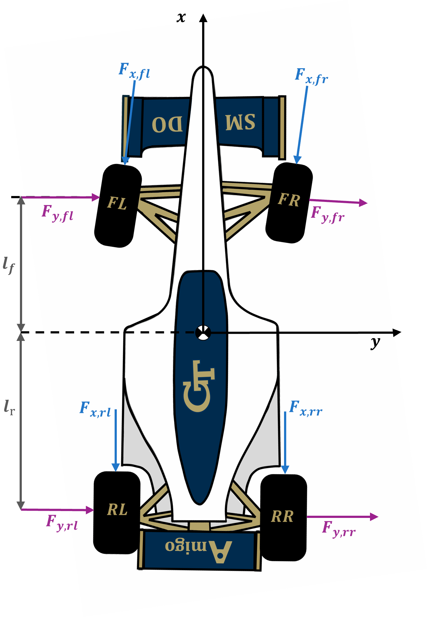
Figure 3. Point mass vehicle model simplification.

Double-Track Model

The double-track layout treats all four wheels independently, which is essential for capturing the asymmetric tire loading that occurs during combined cornering and acceleration. Each wheel generates its own longitudinal force \(F_{x,ij}\) and lateral force \(F_{y,ij}\), where the first index \(i \in \{f, r\}\) denotes the front or rear axle and the second index \(j \in \{l, r\}\) distinguishes between the left and right side. The steering angle \(\delta\) acts on the front wheels, while the rear wheels remain aligned with the chassis. The complete free-body diagram is shown in Figure 4. The aerodynamic drag is quadratic in vehicle speed and applied at the center of gravity; aerodynamic side forces, yawing moments, and pitching effects are neglected.

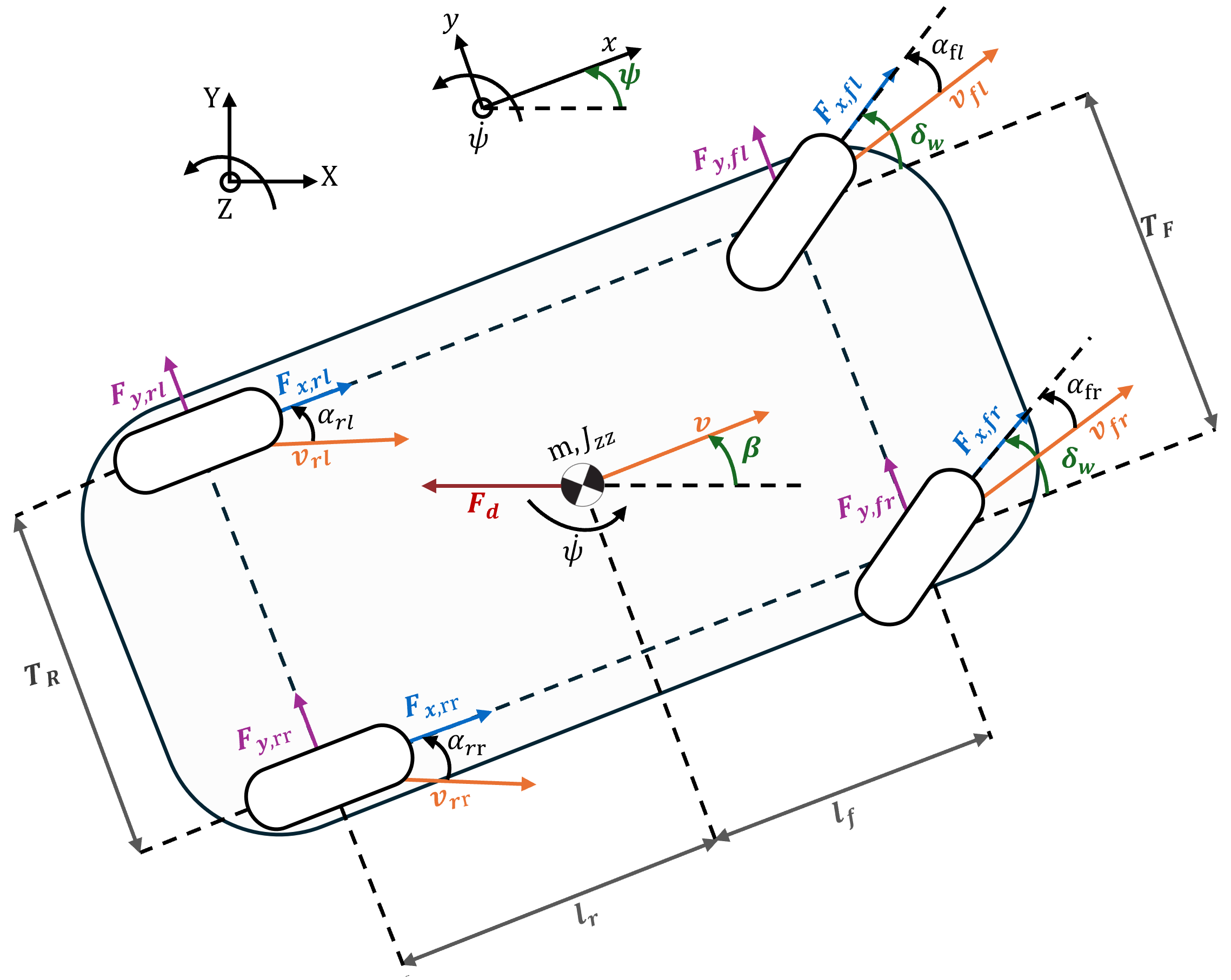
Figure 4. Double-track vehicle model.

State and Control Variables

The dynamics are described by a set of first-order ordinary differential equations. The state variables are:

\[\mathbf{x} = [v, \; \beta, \; \omega_z, \; n, \; \xi]^T\]

Symbol	Description	Unit
\(v\)	Vehicle speed (at the center of gravity)	m/s
\(\beta\)	Body sideslip angle	rad
\(\omega_z\)	Yaw rate	rad/s
\(n\)	Lateral displacement from the reference line	m
\(\xi\)	Relative heading angle	rad

The control variables are:

\[\mathbf{u} = [\delta, \; F_\text{drive}, \; F_\text{brake}, \; \Gamma_y]^T\]

Symbol	Description	Unit
\(\delta\)	Front steering angle	rad
\(F_\text{drive}\)	Total driving force (\(\geq 0\))	N
\(F_\text{brake}\)	Total braking force (\(\leq 0\))	N
\(\Gamma_y\)	Lateral load transfer force	N

The splitting of the longitudinal force into separate driving and braking variables avoids the need for non-smooth functions to distinguish between acceleration and deceleration. To prevent simultaneous braking and driving, the mutual exclusion constraint is enforced:

\[F_\text{drive} \cdot F_\text{brake} = 0 \; \text{N}^2\]

In practice, this complementarity condition is relaxed to an inequality constraint for numerical tractability.

Equations of Motion

The three dynamic equations govern the longitudinal, lateral, and yaw motion about the center of gravity. Define the total axle forces:

\[F_{x}^R = F_{x,rl} + F_{x,rr}, \qquad F_{y}^R = F_{y,rl} + F_{y,rr}\]

\[F_{x}^F = F_{x,fl} + F_{x,fr}, \qquad F_{y}^F = F_{y,fl} + F_{y,fr}\]

and the aerodynamic drag \(F_\text{drag} = \tfrac{1}{2} c_d \rho A v^2\).

Longitudinal Acceleration

\[\dot{v} = \frac{1}{m} \Big[ F_{x}^R \cos\beta + F_{x}^F \cos(\delta - \beta) + F_{y}^R \sin\beta - F_{y}^F \sin(\delta - \beta) - F_\text{drag}\cos\beta \Big]\]

Sideslip Rate

\[\dot{\beta} = -\omega_z + \frac{1}{mv} \Big[ -F_{x}^R \sin\beta + F_{x}^F \sin(\delta - \beta) + F_{y}^R \cos\beta + F_{y}^F \cos(\delta - \beta) + F_\text{drag}\sin\beta \Big]\]

The \(-\omega_z\) term accounts for the rotation of the body frame.

Yaw Acceleration

\[\dot{\omega}_z = \frac{1}{J_{zz}} \bigg[ \underbrace{(F_{x,rr} - F_{x,rl})\frac{t_{w,r}}{2}}_{\text{rear longitudinal}} - \underbrace{F_{y}^R \, l_r}_{\text{rear lateral}} + \underbrace{\Big((F_{x,fr} - F_{x,fl})\cos\delta + (F_{y,fl} - F_{y,fr})\sin\delta\Big)\frac{t_{w,f}}{2}}_{\text{front track-width moment}} + \underbrace{\Big(F_{y}^F \cos\delta + F_{x}^F \sin\delta\Big) l_f}_{\text{front axle moment}} \bigg]\]

Here \(m\) is the vehicle mass, \(J_{zz}\) the yaw inertia, \(l_f\)/\(l_r\) the CG-to-axle distances, and \(t_{w,f}\)/\(t_{w,r}\) the front/rear track widths.

Curvilinear Kinematics

Combined with the curvilinear kinematics from Section 2.1, the lateral displacement and heading evolve in the arc-length domain as:

\[\frac{dn}{ds} = v \sin(\xi + \beta) \cdot S_F\]

\[\frac{d\xi}{ds} = \omega_z \cdot S_F - \kappa\]

The curvature \(\kappa\) is subtracted because the centerline reference frame itself rotates along the track.

Longitudinal Tire Forces

The braking and driving forces are distributed to the individual wheels via static distribution coefficients \(k_\text{drive}\) and \(k_\text{brake}\):

\[F_{x,fj} = \tfrac{1}{2} k_\text{drive} F_\text{drive} + \tfrac{1}{2} k_\text{brake} F_\text{brake} - \tfrac{1}{2} f_r m g \frac{l_r}{L}\]

\[F_{x,rj} = \tfrac{1}{2} (1 - k_\text{drive}) F_\text{drive} + \tfrac{1}{2} (1 - k_\text{brake}) F_\text{brake} - \tfrac{1}{2} f_r m g \frac{l_f}{L}\]

where \(j \in \{l, r\}\) denotes left or right, \(f_r\) is the rolling resistance coefficient, and \(L = l_f + l_r\) is the wheelbase.

Lateral Tire Forces: Extended Pacejka Model

The lateral tire forces are determined using an extended version of Pacejka’s Magic Formula that includes a degressive behavior against the wheel load:

\[F_{y,ij} = \mu_{ij} F_{z,ij} \left(1 + \varepsilon_i \frac{F_{z,ij}}{F_{z0,i}}\right) \sin\!\Big(C_i \arctan\!\big(B_i \alpha_{ij} - E_i (B_i \alpha_{ij} - \arctan(B_i \alpha_{ij}))\big)\Big)\]

The coefficient \(\varepsilon \leq 0\) introduces a degressive tire behavior against the normal load: as the wheel load increases, the friction force grows less than proportionally. This is a critical physical effect, because without it the simple Pacejka model significantly overestimates the lateral force capacity at high normal loads.

The tire slip angles \(\alpha_{ij}\) are computed from kinematic relations:

\[\alpha_{fl/fr} = \delta - \arctan\!\left(\frac{l_f \omega_z + v \sin\beta}{v \cos\beta \mp \tfrac{1}{2} t_{w,f} \omega_z}\right)\]

\[\alpha_{rl/rr} = \arctan\!\left(\frac{l_r \omega_z - v \sin\beta}{v \cos\beta \mp \tfrac{1}{2} t_{w,r} \omega_z}\right)\]

where the upper sign corresponds to the left wheel and the lower sign to the right wheel.

Wheel Normal Loads

The normal loads are computed under a quasi-steady-state assumption that neglects suspension dynamics. They depend on the static weight distribution, longitudinal load transfer from acceleration, aerodynamic downforce, and lateral load transfer:

\[F_{z,fl} = \frac{mgl_r}{2L} - \frac{h_\text{cog}}{2L} m a_x - k_\text{roll} \Gamma_y + \tfrac{1}{2} c_{L,f} q_\text{dyn}\]

\[F_{z,fr} = \frac{mgl_r}{2L} - \frac{h_\text{cog}}{2L} m a_x + k_\text{roll} \Gamma_y + \tfrac{1}{2} c_{L,f} q_\text{dyn}\]

\[F_{z,rl} = \frac{mgl_f}{2L} + \frac{h_\text{cog}}{2L} m a_x - (1 - k_\text{roll}) \Gamma_y + \tfrac{1}{2} c_{L,r} q_\text{dyn}\]

\[F_{z,rr} = \frac{mgl_f}{2L} + \frac{h_\text{cog}}{2L} m a_x + (1 - k_\text{roll}) \Gamma_y + \tfrac{1}{2} c_{L,r} q_\text{dyn}\]

where \(q_\text{dyn} = \tfrac{1}{2}\rho A v^2\) is the dynamic pressure times frontal area, \(h_\text{cog}\) is the center of gravity height, \(k_\text{roll}\) is the roll moment distribution (fraction at front axle), and \(c_{L,f}\), \(c_{L,r}\) are the front and rear aerodynamic downforce coefficients.

The approximate longitudinal acceleration entering the load transfer is:

\[m a_x \approx F_\text{drive} + F_\text{brake} - F_\text{drag} - f_r m g\]

The lateral load transfer variable \(\Gamma_y\) must satisfy the equilibrium:

\[\Gamma_y = \frac{h_\text{cog}}{\bar{t}_w} \Big(F_{y,rl} + F_{y,rr} + (F_{x,fl} + F_{x,fr})\sin\delta + (F_{y,fl} + F_{y,fr})\cos\delta\Big)\]

where \(\bar{t}_w = \tfrac{1}{2}(t_{w,f} + t_{w,r})\) is the mean track width. This is enforced as an equality constraint in the optimization.

Variable Tyre-Road Friction Coefficients

Approaches found in literature assume a constant tyre-road friction coefficient \(\mu\) along the racetrack. This assumption represents a drastic simplification in practical application because overestimating the available tyre friction leads directly to safety-critical driving manoeuvres. For this reason, a method is presented which allows a discretised friction map given in Cartesian coordinates \((x_i, y_i, \mu_i)\) to be considered in the OCP.

At each path coordinate \(s_k\), the friction coefficient at each wheel is approximated as a continuous function of the lateral displacement \(n\) using a Gaussian basis function regression:

\[\mu_{ij,k}(s_k) = \sum_{q=1}^{n_\text{gauss}} w_{ij,k,q} \cdot e^{-(n_k - n_q)^2 / 2\sigma^2}\]

where \(w_{ij,k,q}\) are the regression weights, \(\sigma\) is the basis function width, and \(n_q\) are the lateral positions of the basis functions. This representation is well suited for capturing non-uniform variations in friction across the track width.

Optimal Control Problem

Problem Formulation

The formulation of the OCP for the minimum lap time problem is presented in the following general form over the arc-length interval \([s_0, s_f]\):

\[\begin{split}\begin{aligned} \min_{\mathbf{x},\, \mathbf{u}} \quad & \int_{s_0}^{s_f} L\big(\mathbf{x}(s),\, \mathbf{u}(s)\big) \, ds & & \text{(objective)} \\[6pt] \text{s.t.} \quad & \frac{d\mathbf{x}}{ds} = \mathbf{f}\big(\mathbf{x}(s),\, \mathbf{u}(s)\big), & & \text{(dynamics)} \\[6pt] & \mathbf{g}\big(\mathbf{x}(s),\, \mathbf{u}(s)\big) = \mathbf{0}, & & \text{(equality constraints)} \\[6pt] & \mathbf{h}\big(\mathbf{x}(s),\, \mathbf{u}(s)\big) \leq \mathbf{0}, & & \text{(inequality constraints)} \\[6pt] & \mathbf{r}\big(\mathbf{x}(s_0),\, \mathbf{x}(s_f)\big) = \mathbf{0}. & & \text{(boundary conditions)} \end{aligned}\end{split}\]

The state vector \(\mathbf{x}(s) \in \mathbb{R}^{5}\) and control vector \(\mathbf{u}(s) \in \mathbb{R}^{4}\) are as defined in Section 3.3. Each component of this formulation is detailed in the following subsections.

Objective Function

The objective is to minimize the total lap time. Since arc-length \(s\) is the independent variable, the lap time is recovered by integrating the slowness factor:

\[J = \int_{s_0}^{s_f} S_F(s) \, ds, \qquad S_F = \frac{1 - n\,\kappa}{v\cos(\xi + \beta)}\]

A control regularization term is added to penalize large variations between consecutive mesh points and promote smooth inputs:

\[J_\text{reg} = r_\delta \sum_{k=0}^{N-1} (\delta_{k+1} - \delta_k)^2 \;+\; r_F \sum_{k=0}^{N-1} (F^*_{k+1} - F^*_k)^2\]

where \(F^* = F_\text{drive} + F_\text{brake}\) is the net longitudinal force and \(r_\delta\), \(r_F\) are small penalty weights. The total cost is \(J_\text{total} = J + J_\text{reg}\).

Equality Constraints

The equality constraints \(\mathbf{g}(\mathbf{x}, \mathbf{u}) = \mathbf{0}\) enforce algebraic relations that must hold at each mesh point.

Lateral Load Transfer Equilibrium

The control variable \(\Gamma_y\) must satisfy the lateral force balance (Section 3.7):

\[\Gamma_y - \frac{h_\text{cog}}{\bar{t}_w} \Big(F_{y,rl} + F_{y,rr} + (F_{x,fl} + F_{x,fr})\sin\delta + (F_{y,fl} + F_{y,fr})\cos\delta\Big) = 0\]

Mutual Exclusion of Driving and Braking

Simultaneous throttle and brake application is prevented by the complementarity condition:

\[F_\text{drive} \cdot F_\text{brake} = 0\]

In practice this is relaxed to \(F_\text{drive} \cdot F_\text{brake} \leq \epsilon\) for a small tolerance \(\epsilon > 0\).

Inequality Constraints

The inequality constraints \(\mathbf{h}(\mathbf{x}, \mathbf{u}) \leq \mathbf{0}\) enforce the physical limits of the vehicle at each mesh point.

Kamm’s Friction Circle

The combined tire force at each wheel must not exceed the friction limit:

\[F_{x,ij}^2 + F_{y,ij}^2 \leq (\mu_{ij} \, F_{z,ij})^2, \qquad ij \in \{fl,\, fr,\, rl,\, rr\}\]

Engine Power Limit

The driving power is bounded by the maximum available power:

\[v \cdot F_\text{drive} \leq P_\text{max}\]

Actuator Rate Constraints

Control rates are limited to reflect physical actuator dynamics, using the local time step \(\Delta t_k = S_{F,k} \cdot \Delta s\):

\[\left|\frac{\delta_{k+1} - \delta_k}{\Delta t_k}\right| \leq \frac{\delta_\text{max}}{T_\delta}, \qquad \frac{F_{\text{drive},k+1} - F_{\text{drive},k}}{\Delta t_k} \leq \frac{F_\text{drive,max}}{T_\text{drive}}, \qquad \frac{-(F_{\text{brake},k+1} - F_{\text{brake},k})}{\Delta t_k} \leq \frac{|F_\text{brake,min}|}{T_\text{brake}}\]

where \(T_\delta\), \(T_\text{drive}\), and \(T_\text{brake}\) are actuator time constants.

Track Boundary Constraints

The vehicle must remain within the road boundaries:

\[-N_r(s) + \frac{b_\text{veh}}{2} \;\leq\; n(s) \;\leq\; N_l(s) - \frac{b_\text{veh}}{2}\]

Boundary Conditions

The track is a closed loop, so the solution must satisfy periodic boundary conditions:

\[\mathbf{r}\big(\mathbf{x}(s_0),\, \mathbf{x}(s_f)\big) = \mathbf{x}(s_0) - \mathbf{x}(s_f) = \mathbf{0}\]

Variable Bounds

The state and control variables are subject to box constraints (Table A1 of [1]):

Variable	Lower bound	Upper bound
\(v\)	1 m/s	\(v_\text{max}\)
\(\beta\)	\(-\pi/2\)	\(\pi/2\)
\(\omega_z\)	\(-2\) rad/s	\(2\) rad/s
\(n\)	\(-(w_r - b_\text{veh}/2)\)	\(w_l - b_\text{veh}/2\)
\(\xi\)	\(-\pi/2\)	\(\pi/2\)
\(\delta\)	\(-\delta_\text{max}\)	\(\delta_\text{max}\)
\(F_\text{drive}\)	0	\(F_\text{drive,max}\)
\(F_\text{brake}\)	\(F_\text{brake,min}\)	0

The lower bound on velocity prevents a singularity in \(S_F\) when \(v \to 0\).

Vehicle Parameters

The vehicle parameters correspond to a Formula E class racing car (Table A1 of [1]):

Parameter	Symbol	Value	Unit
Vehicle mass	\(m\)	1200	kg
CG to front axle	\(l_f\)	1.5	m
CG to rear axle	\(l_r\)	1.4	m
Track width, front	\(t_{w,f}\)	1.6	m
Track width, rear	\(t_{w,r}\)	1.5	m
Vehicle width	\(b_\text{veh}\)	2.0	m
CG height	\(h_\text{cog}\)	0.4	m
Yaw moment of inertia	\(J_{zz}\)	1260	kg m\(^2\)
Frontal area	\(A\)	1.0	m\(^2\)
Drag coefficient	\(c_d\)	1.4	–
Downforce coeff., front	\(c_{L,f}\)	2.4	–
Downforce coeff., rear	\(c_{L,r}\)	3.0	–
Rolling resistance coeff.	\(f_r\)	0.010	–
Air density	\(\rho\)	1.2041	kg/m\(^3\)
Max engine power	\(P_\text{max}\)	270	kW
Max driving force	\(F_\text{drive,max}\)	7100	N
Max braking force	\(F_\text{brake,min}\)	$-$20000	N
Max steering angle	\(\delta_\text{max}\)	0.4	rad
Max velocity	\(v_\text{max}\)	42.5	m/s
Drive force distribution	\(k_\text{drive}\)	0.0 (RWD)	–
Brake force distribution	\(k_\text{brake}\)	0.7	–
Roll moment distribution	\(k_\text{roll}\)	0.5	–

Pacejka Tire Parameters

The tire parameters for the extended Pacejka model (Table A2 of [1]):

Parameter	Front	Rear
Stiffness factor \(B\)	9.62	8.62
Shape factor \(C\)	2.59	2.65
Curvature factor \(E\)	1.0	1.0
Nominal load \(F_{z0}\) (N)	3000	3000
Load degression \(\varepsilon\)	-0.0813	-0.1263
Friction coefficient \(\mu\)	1.0	1.0

Numerical Method

The continuous OCP is transcribed into a finite-dimensional nonlinear program (NLP) using direct collocation. The track is divided into \(N\) intervals of equal arc length \(\Delta s = s_f / N\), with nodes \(s_k = k \cdot \Delta s\) for \(k = 0, \ldots, N\). At each node the decision variables are \(\mathbf{x}_k \in \mathbb{R}^{5}\) and \(\mathbf{u}_k \in \mathbb{R}^{4}\), giving a total of \(9N\) NLP variables.

The dynamics are enforced through trapezoidal collocation defect constraints:

\[\mathbf{x}_{k+1} - \mathbf{x}_k - \frac{\Delta s}{2}\Big(\mathbf{f}(\mathbf{x}_k, \mathbf{u}_k, \kappa_k) + \mathbf{f}(\mathbf{x}_{k+1}, \mathbf{u}_k, \kappa_{k+1})\Big) = \mathbf{0}, \qquad k = 0, \ldots, N-1\]

The objective is discretized with the same rule:

\[J = \sum_{k=0}^{N-1} \frac{\Delta s}{2} \big( S_{F,k} + S_{F,k+1} \big) + J_\text{reg}\]

The complete NLP constraint structure at each node is summarized below:

Constraint	Type	Count
Defect: \(\mathbf{x}_{k+1} - \mathbf{x}_k - \frac{\Delta s}{2}(\mathbf{f}_k + \mathbf{f}_{k+1}) = 0\)	Equality	5
Lateral load transfer equilibrium	Equality	1
Mutual exclusion: \(F_\text{drive} \cdot F_\text{brake} = 0\)	Equality	1
Kamm’s circle (4 wheels)	Inequality	4
Engine power	Inequality	1
Track boundaries	Bounds	2
Actuator rates	Inequality	3
Variable bounds	Bounds	9

The periodic boundary condition \(\mathbf{x}_0 = \mathbf{x}_N\) closes the loop. The resulting sparse NLP is solved using a large-scale nonlinear programming solver.

Assignment

The goal of this project is to implement and solve the minimum lap time problem described in the preceding sections. The assignment is divided into the following tasks:

1. Model implementation: Implement the full double-track vehicle model (Sections 3 to 4) as a nonlinear optimal control problem. The implementation should cover the state dynamics, tire and load transfer models, all constraints, boundary conditions, and the collocation scheme as described in Sections 3 to 7. Use the vehicle and tire parameters from Sections 5 and 6.

2. Choice of software framework: You may use either Amigo or Dymos for this project. This problem produces a large, sparse NLP with thousands of variables and constraints, and therefore requires a large-scale NLP solver capable of exploiting sparsity together with automatic differentiation for exact first-order, and ideally second-order, derivatives. Note that while Dymos can use SciPy optimizers, a problem of this size and complexity requires a high-performance large-scale NLP solver (e.g. IPOPT), which can be difficult to install, particularly on Windows where building from source with performant linear solvers (e.g. HSL) requires substantial effort. We recommend Amigo, which ships with a built-in large-scale interior-point solver, compiled C++ backend, and exact second-order AD. To get started with Amigo, documentation and trajectory optimization tutorials are available here. The documentation is actively maintained and expanded. A starter code implementing a simplified single-track version of the lap time problem will be provided for Amigo users as a reference to help you get up to speed with the framework. An equivalent example using an oval track is also available for Dymos here.

3. Track data and optimization: The optimization must be conducted on two tracks:

(a) Berlin Formula E circuit: The Berlin 2018 Formula E circuit used in [1]. The preprocessed track data (centerline coordinates and track widths) is available at:

github.com/TUMFTM/global_racetrajectory_optimization/…/berlin_2018.csv

A track processing code will be provided that loads the CSV data, computes the arc-length parametrization and curvature \(\kappa(s)\), applies Gaussian smoothing, and resamples onto a uniform mesh with interpolated track widths \(N_l(s)\) and \(N_r(s)\). Your task is to replace the Gaussian smoothing with a spline-based approach, which produces a smoother and more differentiable curvature profile, important since \(\kappa(s)\) enters directly into the dynamics. You may use either scikit-learn or scipy.interpolate for the spline regression. The smoothing parameter controls the trade-off between fidelity to the raw data and smoothness. Apply your spline-based smoothing to both tracks.

(b) Circuit of your choice: Select a second circuit from the Formula 1 circuit database:

github.com/bacinger/f1-circuits

This repository provides circuit layouts in GeoJSON format. Unlike the Berlin data, no preprocessed centerline or track widths are provided. You will need to parse the GeoJSON geometry, convert geographic coordinates (longitude, latitude) to a local Cartesian frame, and estimate a constant track width (a reasonable assumption is 10 to 15 m for F1 circuits, or research the actual width for your chosen track). The same track processing utility can be adapted for this purpose, using the spline-based curvature smoothing from Task 3(a).

Report Requirements

Write a five-page report with a 300-word abstract. You may use the AIAA paper format if you wish. Keep your descriptions concise and make your plots clear with labels and concise captions.

1. Problem formulation: Write out a description of the optimal control problem formulation, including the objective, state dynamics, and all constraints. Clearly define the state and control variables and explain how the continuous OCP is transcribed into a finite-dimensional NLP via direct collocation.

2. Track data processing: Describe your approach for processing the track data. For each track, plot the raw and smoothed curvature profiles For each track, show the raw curvature alongside the spline-smoothed curvature and discuss your choice of smoothing parameter. Show the track layout with the computed centerline and boundaries.

3. Vehicle model verification: Describe your implementation of the vehicle model. Plot the tire force characteristics (Pacejka curves) for the front and rear tires across a range of slip angles and normal loads. Verify that Kamm’s friction circle is respected at all four wheels in the optimal solution.

4. Optimization results: For each track, report the optimal lap time \(T_\text{lap}\) and present plots of the optimal racing line, velocity profile, tire utilization (Kamm’s circle), and steering/throttle/brake inputs along the track.

5. Challenges and modifications: Describe issues you found with your optimization. What was successful? What modifications did you make? How did you overcome any challenges (e.g. initialization strategy, solver convergence, regularization tuning, mesh refinement)?

6. Comparative analysis: Compare the results from both tracks. Discuss how track characteristics (curvature distribution, straight lengths, corner sequences) influence the optimal driving strategy. Compare optimal lap times, maximum speeds, and minimum corner speeds. Include an assessment of solver performance: number of iterations, convergence behavior, and computation time.

References

1. Christ, F., Wischnewski, A., Heilmeier, A., & Lohmann, B. (2021). Time-optimal trajectory planning for a race car considering variable tyre-road friction coefficients. Vehicle System Dynamics, 59(4), 588–612.

2. Casanova, D. (2000). On Minimum Time Vehicle Manoeuvring: The Theoretical Optimal Lap. PhD thesis, Cranfield University.

3. Kelly, D. P. (2008). Lap Time Simulation with Transient Vehicle and Tyre Dynamics. PhD thesis, Cranfield University.

4. Perantoni, G., & Limebeer, D. J. N. (2014). Optimal control for a Formula One car with variable parameters. Vehicle System Dynamics, 52(5), 653–678.

5. Dal Bianco, N., Lot, R., & Gadola, M. (2018). Minimum time optimal control simulation of a GP2 race car. Proceedings of the Institution of Mechanical Engineers, Part D: Journal of Automobile Engineering, 232(9), 1180–1195.

6. Pacejka, H. B. (2012). Tire and Vehicle Dynamics (3rd ed.). Butterworth-Heinemann.

7. Wachter, A., & Biegler, L. T. (2006). On the implementation of an interior-point filter line-search algorithm for large-scale nonlinear programming. Mathematical Programming, 106(1), 25–57.