Multidisciplinary Optimization
Multidisciplinary Optimization (MDO) is a field of study that comprises a number of methods that are designed to both (1) couple multiple disciplines together to perform an analysis of a complex engineering system, and (2) optimize the engineering system.
MDO is an important special case of simulation-based optimization.
There are two key challenges in MDO:
The analysis problem in MDO: How should MDO algorithms ensure that the inputs and outputs of each discipline are compatible with each other so that the multidisciplinary analysis is self-consistent?
The optimization problem in MDO: How should MDO algorithms optimize the multidisciplinary system?
MDO algorithms address both the analysis part of the MDO problem and the optimization part of the MDO problem in different ways. Some tackle these two problems in sequence while others attempt to tackle them concurrently.
In MDO methods, disciplinary feasibility is achieved when the inputs from one discipline are specified and used to generate that discipline’s converged output values. Disciplinary feasibility may be violated if your discipline solver is complex and requires many iterations to converge. In this case, you may not want to converge the discipline solver to a tight tolerance before considering coupling from other disciplines. For instance, it may be beneficial to partially converge a CFD solution, predict aerodynamic loads for the structural analysis and then evaluate new structural and aerodynamic displacements. This may save computational time in the end, but the discipline is not yet converged so disciplinary feasibility is not achieved.
Multidisciplinary feasibility is achieved when we have disciplinary feasibility for all disciplines and the inputs and outputs of all disciplines agree.
A complete overview of MDO architectures is beyond the scope of this course. I recommend you read the paper: “Multidisciplinary Design Optimization: A Survey of Architectures” available here:
https://arc.aiaa.org/doi/10.2514/1.J051895
The methods and techniques in this paper summarize work on MDO methods before 2013. But modern approaches tend not to fit neatly into one of these architectures.
To make the results in this section more concrete, we will look at performing a static aeroelastic simulation and optimization problem.
Multidisciplinary analysis case study: Aeroelastic analysis
Consider the design of a flexible aircraft wing. In flight, the wing is in equilibrium so that the aerodynamic and inertial forces balance with the internal structural forces. The deformation of the structure matches the flying outer-mold-line of the wing surface.
In many aircraft, the deformation is large enough that there is a significant difference between the jig shape of the wing and the flying shape. We want to analyze the wing and optimize it for its flying shape, not the shape that it is built it in.
To determine the flying shape of the wing, as well as the lift and drag produced by the deformed wing, we have to consider both the aerodynamics and structures together. The aerodynamics constitutes one discipline and the structures constitute a second discipline. These disciplines must be considered together.
Components of Aeroelastic Analysis and Design Optimization
Aeroelastic couples aerodynamic forces with structural deformations. In addition, there are issues that must be addressed including transfer of aerodynamic forces to a structural mesh and passing structural deformations to the aerodynamic surface.
Furthermore, we need to define what are our design variables and functions of interest that will serve as either objectives or constraints.
Geometry input
The geometry of the wing specifies the initial aerodynamic surface and geometry of the wing structure. In this instance, we will use a beam model for the wing and a mid-surface model for the wing. The geometry will be responsible for generating the initial wing mesh, including mesh node locations.
The geometry variables will be a subset of the design variables \(x\) and will be used to generate the aerodynamic node locations, control points and surface normals that we’ll generically denote as \(x_{A0}\). This geometry dependence is explicit, in the sense that it does not require the solution of a system of equations, and can be written as follows
Here \(x_{A0}\) is used since this is the initial, undeformed wing configuration. Later, we will add an additional computation to the code to compute the true deformed shape of the wing. This deformed geometry will be denoted \(x_{A}\).
The geometry variables will also be used to compute the structural node locations \(x_S\). This will be denoted as
Aerodynamic Analysis
The aerodynamic analysis will consist of a Weissinger model of the wing. This consists of a system of horseshoe vortices that are placed along the 1/4 chord of the wing. Boundary conditions that impose no normal flow through the wing are imposed at the 3/4 chord point.
The aerodynamic model depends on the deformed aerodynamic geometry \(x_{A}\) as well as the angle of attack \(\alpha\) and the onset velocity \(V_{\infty}\) that we place in the design vector \(x\). The aerodynamic analysis is implicit since it involves solving a linear system of equations to obtain the aerodynamic states \(\Gamma\).
The aerodynamic states represent the circulation of each of the horseshoe vortices on the wing.
The aerodynamic forces have to be computed after we obtain a solution of the aerodynamic governing equations. This computation takes the form
Note that this computation also depends on the angle of attack and onset velocity.
Structural Analysis
The structural analysis consists of a simple beam model that is placed at the 1/4 chord line of the wing. We use a straightforward linear beam model where the stiffness matrix depends on the structural node locations and the beam properties denoted as \(x_{B}\).
The relationship between the beam properties \(x_{B}\) such as axial, torsional and bending stiffness and the design variables depends on the type of model used. These stiffness properties can be computed as a direct function of the design variables usign the explicit relationship
Once the beam properties have been computed, we can form the implicit finite-element governing equations for the beam as
Here \(K\) is the stiffness matrix and \(f_{S}\) are the structural forces and \(u_{S}\) are the structural displacements.
Load and Discplacement Transfer
The aerodynamic geometry must be moved to its deformed state. To perform this task, we require a displacement transfer scheme that will give the aerodynamic shape as a function of the structural displacements. These methods may be implicit or explicit. In this example problem, we use an explicit displacement transfer technique that can be written as follows:
The loads computed by the aerodynamics must be transferred to loads on the structural mesh. Like the displacement transfer scheme, the approach used here is explicit and can be written as
In general, the load and displacement transfer schemes are typically closely related via the method of virtual work. This ensures that the work done by the aerodynamic forces on the displaced aerodynamic mesh is equal to the work done on the structures with the structural forces moving through the structural displacements.
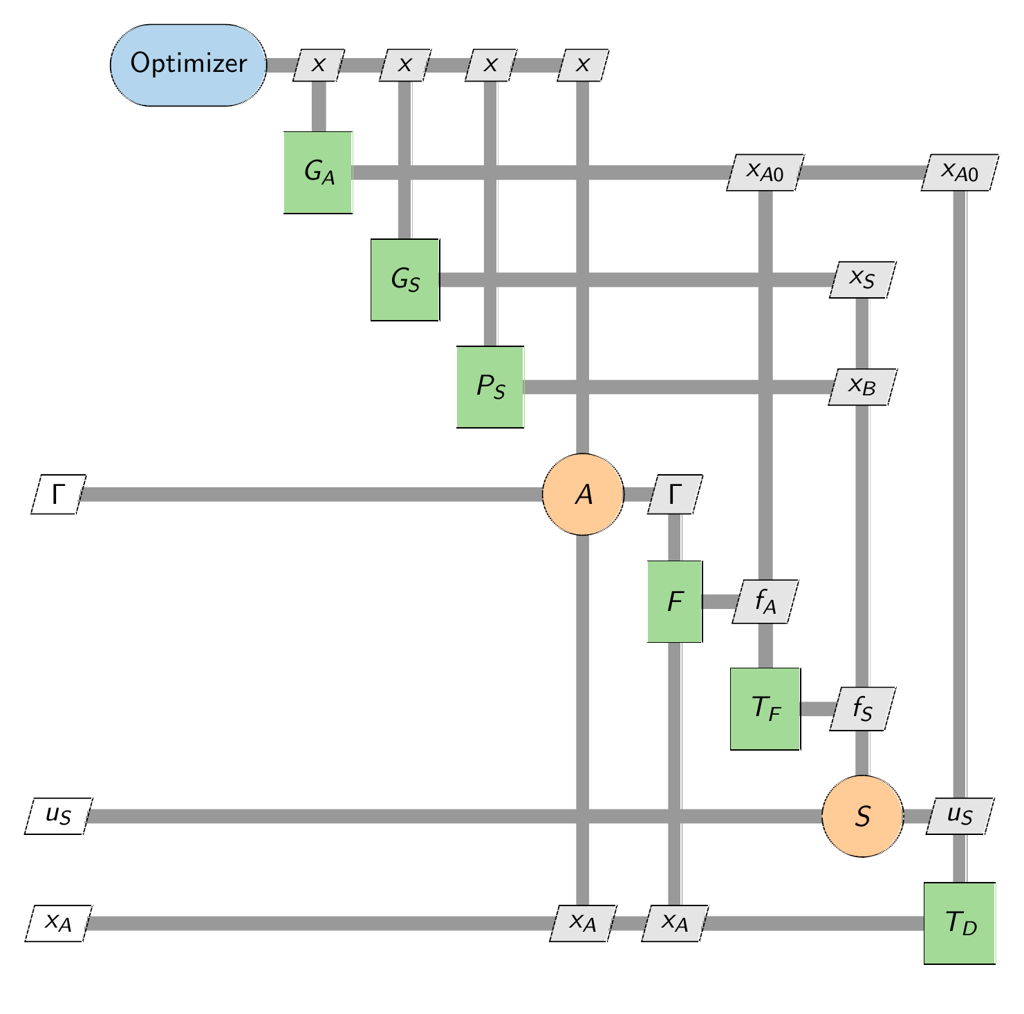
Multidisciplinary Feasible Architecture
In the Multidisciplinary Feasible (MDF) MDO Architecture, a multidiscipline feasible solution of the multidisciplinary system is found at each new design point. We will then use the adjoint method to compute the gradient of functions of interest and use an optimizer to optimize the system performance. MDF is a direct application of the reduced-space method from simulation based optimization.
For the aeroelastic system, we can make some observations. Given the design variables \(x\), we can immediately compute \(x_{S} = G_{S}(x)\), \(x_{A0} = G_{A}(x)\) and \(x_{B} = P(x)\). However, we still need to compute the solution of the remaining governing equations that when concatenated take the form
where we will solve for \(\Gamma\), \(f_{A}\), \(f_{S}\), \(u_{S}\) and \(x_{A}\), treating \(x_{S}\), \(x_{A0}\) and \(x_{B}\) as fixed.
Nonlinear block Gauss-Seidel method
We can solve the coupled system of equations by using a nonlinear block Gauss-Seidel method. In this technique, we solve the coupled linear system by sequentially going through each of the component analyses and computing the required solution. In this example, this would lead to the following sequence of steps, taking \(x_{A} = x_{A0}\):
Solve \(A(x, x_{A}, \Gamma) = 0\) for \(\Gamma\)
Compute the aerodynamic forces \(f_{A} = F(x, x_{A}, \Gamma)\)
Transfer the aerodynamic forces to the structures \(f_{S} = T_{F}(f_{A}, x_{A0}, x_{S})\)
Solve \(S(x_{B}, x_{S}, u_{S}, f_{S}) = 0\) for \(u_{S}\)
Transfer the displacements to the \(x_{A} = T_{D}(u_{S}, x_{A0}, x_{S})\)
This loop iterates until convergence.
The problem with NLBGS methods is that they can be slow to converge. Different damping strategies can be used to try and make the iteration more robust or potentially faster to converge.
Newton method
Newton’s method can also be used to converge the multidisciplinary system of equations. This takes the form
MDF Adjoint
Given a generic function of the form \(f(\Gamma, u_{S}, x_{A})\), the MDF adjoint takes the form
Once the adjoint variables have been obtained, you can compute the total derivative
Linear Block Gauss-Seidel Adjoint method
The adjoint system can be solved using the following sequence of steps:
Solve \(\left[ \partial_{u_{S}} S \right]^{T} \psi_{u_{S}} = - \partial_{u_{S}} f + \left[ \partial_{u_{S}} T_{D} \right]^{T} \psi_{x_{A}}\)
Compute \(\psi_{f_{S}} = - \left[ \partial_{f_{S}} S \right]^{T} \psi_{u_{S}}\)
Compute \(\psi_{f_{A}} = \left[ \partial_{f_{A}} T_{F} \right]^{T} \psi_{f_{S}}\)
Solve \(\left[ \partial_{\Gamma} A \right]^{T} \psi_{\Gamma} = - \partial_{\Gamma} f + \left[ \partial_{\Gamma} F \right]^{T} \psi_{f_{A}}\)
Compute \(\psi_{x_{A}} = -\partial_{x_{A}} f + \left[ \partial_{x_{A}} F \right]^{T} \psi_{f_{A}} - \left[ \partial_{x_{A}} A \right]^{T} \psi_{\Gamma}\)
XDSM Diagrams: Visualizing and representing MDO problems
An eXtended Design Structure Matrix (XDSM) diagram illustrates the connections between disciplines and the execution of an MDO algorithm. It is convenient way to depict the flow of information within a complex multidisciplinary system.
https://link.springer.com/article/10.1007/s00158-012-0763-y
[2]:
from pyxdsm.XDSM import XDSM, OPT, SOLVER, FUNC, LEFT
from pdf2image import convert_from_path

# Change `use_sfmath` to False to use computer modern
x = XDSM(use_sfmath=True)

x.add_system("opt", OPT, r"\text{Optimizer}")

x.add_system("aero_geo", FUNC, "G_{A}")
x.add_system("struct_geo", FUNC, "G_{S}")
x.add_system("struct_props", FUNC, "P_{S}")
x.add_system("aero", SOLVER, "A")
x.add_system("force", FUNC, "F")
x.add_system("transfer_f", FUNC, "T_{F}")
x.add_system("struct", SOLVER, "S")
x.add_system("transfer_u", FUNC, "T_{D}")

# Connect the design variables
x.connect("aero_geo", "transfer_f", "x_{A0}")
x.connect("aero_geo", "transfer_u", "x_{A0}")
x.connect("opt", "aero", "x")
x.connect("opt", "aero_geo", "x")
x.connect("opt", "struct_geo", "x")
x.connect("opt", "struct_props", "x")
x.connect("struct_geo", "struct", "x_{S}")
x.connect("struct_props", "struct", "x_{B}")

# Connect the state variables
x.connect("aero", "force", r"\Gamma")
x.connect("force", "transfer_f", "f_{A}")
x.connect("transfer_f", "struct", "f_{S}")
x.connect("struct", "transfer_u", "u_{S}")
x.connect("transfer_u", "aero", "x_A")
x.connect("transfer_u", "force", "x_A")

# Outputs
x.add_output("aero", r"\Gamma", side=LEFT)
x.add_output("struct", r"u_{S}", side=LEFT)
x.add_output("transfer_u", r"x_{A}", side=LEFT)

x.write("mdf", quiet=True)

images = convert_from_path("mdf.pdf", dpi=300)
images[0].save("mdf.png")
This is pdfTeX, Version 3.141592653-2.6-1.40.27 (TeX Live 2025) (preloaded format=pdflatex)
 restricted \write18 enabled.
entering extended mode
OpenMDAO: Complex multidisciplinary problems
OpenMDAO is a framework for implementing and solving multidisciplinary optimization problems.
There are a lot of resources for OpenMDAO and an active community for development and support.
You can use pip to install OpenMDAO. I recommend this approach. Simply type pip install openmdao. We’ll also use Dymos that is built pip install dymos.
The theory behind OpenMDAO is described in this paper:
https://link.springer.com/article/10.1007/s00158-019-02211-z
Implicit and explicit component types
In an OpenMDAO model, you build a system from one or more components. The components are either of type ExplicitComponent that directly define outputs in terms of inputs, or are of type ImplicitComponent that solve an implicit system of equations to determine their outputs in terms of inputs. The interfaces that are required for ExplicitComponent and ImplicitComponent are different.
I recommend that you use ExplicitComponent as much as possible, and use the ImplicitComponent type only when required.
There are many examples on the OpenMDAO website of how to build these component types. I recommend these simple examples as a starting point:
Here’s some of the basics. Both the ExplicitComponent and ImplicitComponent types require the same basic definitions:
Define an
def initialize(self):function where you declare options that will be arguments to your class when you create it. These options can have defaults.
Put calls to
self.options.declare(...)here
Define a
def setup(self):function that declares inputs and outputs for your component.
Call
self.add_input("name", val=)to specify the name and initial value of any inputsCall
self.add_output("name", val=)to specify the name and initial value of ouptuts
Define a
def setup_partials(self):function that declares the partial derivatives that your component defines and how they will be computed. You can use either exact methods, where you implement the derivative yourself, or the finite-difference or complex-step method to approximate the derivatives.
Call
self.declare_partial(of="output", wrt="input", method="exact" | "cs" | "fd")to declare the derivatives you’ll use.
The ExplicitComponent type also requires that you define two additional functions:
def compute(self, inputs, outputs):Computes theoutputsbased on the values stored in theinputs.
outputs["area"] = np.pi * inputs["radius"] ** 2
def compute_partials(self, inputs, partials):Computes the partial derivatives you declared
partials["area", "radius"] = 2.0 * np.pi * inputs["radius"]
The ImplicitComponent type also requires that you define two additional functions (and optionally some more defined in the OpenMDAO pages):
def apply_nonlinear(self, inputs, outputs, residuals):Computes the residuals given the inputs, the guess for the outputs. The residuals are associated with the outputs defined by theImplicitComponent.
residuals["u_S"] = K.dot(outputs["u_S"]) - inputs["f_S"]Compute the residual \(r = K u_{S} - f\).
def solve_nonlinear(self, inputs, outputs):Solves the possibly nonlinear residuals to obtain the outputs in terms of the inputs.
outputs["u_S"] = np.linalg.solve(K, inputs["f_S"])Computes \(u_{S} = K^{-1} f\).
Connecting components
An isolated component may not do what you need. It can be helpful to build large complex simulations as collections of components.
There are a number of ways to connect the inputs from one component to the outputs of another. A simple example of this is by explicitly connecting them with the connect function. The name of a component gets prepended to the name of the variable. Therefore, to connect a semi_span variable from one component to another might look like this:
# Create an empty OpenMDAO problem with a model class
prob = om.Problem()

# Create an independent variable component that is the source component for variables.
# Outputs of the IVC get connected to inputs of different components.
indeps = prob.model.add_subsystem("vars", om.IndepVarComp())
indeps.add_output("semi_span", val=10.0, units="m")

# Add a sub-system with a "semi_span" variable output
prob.model.add_subsystem("aero_mesh", AeroMesh(num_aero_pts=10))
prob.model.connect("vars.semi_span", "aero_mesh.semi_span")
You can also connect variables with promotion. This gets a little more complicated. I recommend against using this approach until you’re a knowledgable OpenMDAO user.
Checking partial derivatives
Inaccuracy in the derivatives can lead to problems with your model converging or the optimizer converging. It’s always a good idea to check the partial derivatives of your components individually before you assemble them.
After you’ve completed making connections, you can check partial derivatives as follows
# Finish the problem set up and force all variables to be allocated as complex
prob.setup(force_alloc_complex=True)

# Run the model to propagate inputs to outputs
prob.run_model()

# Perform a partial derivative check on components using a complex-step method. Print a summary of the results.
cpd = prob.check_partials(method="cs", compact_print=True)
[4]:
import numpy as np
import openmdao.api as om

class AeroMesh(om.ExplicitComponent):
    """
    Aerodynamic mesh
    """

    def initialize(self):
        self.options.declare("num_aero_pts", types=int)

        # Set the span direction and the chord direction
        self.span_dir = np.array([0.0, 1.0, 0.0])
        self.chord_dir = np.array([1.0, 0.0, 0.0])

        return

    def setup(self):
        num_aero_pts = self.options["num_aero_pts"]

        # Geometry input variables
        self.add_input("semi_span", val=1.0, units="m")
        self.add_input("root_chord", val=1.0, units="m")
        self.add_input("taper_ratio", val=1.0, units=None)
        self.add_input("sweep", val=0.0, units="deg")

        # Node and control point location outputs
        self.add_output("aero_X0", val=np.zeros((num_aero_pts + 1, 3)), units="m")
        self.add_output("aero_Xcp0", val=np.zeros((num_aero_pts, 3)), units="m")
        self.add_output("aero_ncp0", val=np.zeros((num_aero_pts, 3)), units="m")

        return

    def setup_partials(self):
        # Declare the partials - compute all of these analytically
        all_vars = ["semi_span", "root_chord", "taper_ratio", "sweep"]
        self.declare_partials(of="aero_X0", wrt=all_vars)
        self.declare_partials(of="aero_Xcp0", wrt=all_vars)
        self.declare_partials(of="aero_ncp0", wrt=all_vars)

        return

    def compute(self, inputs, outputs):
        num_aero_pts = self.options["num_aero_pts"]

        semi_span = inputs["semi_span"]
        root_chord = inputs["root_chord"]
        taper_ratio = inputs["taper_ratio"]
        sweep = inputs["sweep"]

        Lambda = np.pi * sweep / 180.0

        # Compute the node locations. These are placed at the 1/4 chord location
        u0 = 2.0 - np.cos(np.pi * np.linspace(0.5, 1.0, num_aero_pts + 1))
        chord0 = root_chord * ((1.0 - u0) + taper_ratio * u0)

        aero_X0 = np.outer(semi_span * u0, self.span_dir)
        aero_X0 += np.outer(0.25 * chord0 + semi_span * u0 * np.tan(Lambda), self.chord_dir)
        outputs["aero_X0"] = aero_X0

        # Compute the control point locations. These are placed at the 3/4 chord location
        delta = 0.25 / num_aero_pts
        ucp = 2.0 - np.cos(np.pi * np.linspace(0.5 + delta, 1.0 - delta, num_aero_pts))
        chordcp = root_chord * ((1.0 - ucp) + taper_ratio * ucp)

        aero_Xcp0 = np.outer(semi_span * ucp, self.span_dir)
        aero_Xcp0 += np.outer(0.75 * chordcp + semi_span * ucp * np.tan(Lambda), self.chord_dir)
        outputs["aero_Xcp0"] = aero_Xcp0

        aero_ncp0 = np.zeros((num_aero_pts, 3))
        aero_ncp0[:, 2] = 1.0
        outputs["aero_ncp0"] = aero_ncp0

        return

    def compute_partials(self, inputs, partials):
        num_aero_pts = self.options["num_aero_pts"]

        semi_span = inputs["semi_span"]
        root_chord = inputs["root_chord"]
        taper_ratio = inputs["taper_ratio"]
        sweep = inputs["sweep"]

        Lambda = np.pi * sweep / 180.0
        dLambdadsweep = np.pi / 180.0

        # Compute the node locations. These are placed at the 1/4 chord location
        u0 = 2.0 - np.cos(np.pi * np.linspace(0.5, 1.0, num_aero_pts + 1))
        dchord0drc = ((1.0 - u0) + taper_ratio * u0)
        dchord0dtr = root_chord * u0

        partials["aero_X0", "semi_span"] = np.outer(u0, self.span_dir) + np.outer(u0 * np.tan(Lambda), self.chord_dir)
        partials["aero_X0", "root_chord"] = np.outer(0.25 * dchord0drc, self.chord_dir)
        partials["aero_X0", "taper_ratio"] = np.outer(0.25 * dchord0dtr, self.chord_dir)
        partials["aero_X0", "sweep"] = np.outer(semi_span * u0 / np.cos(Lambda)**2, self.chord_dir) * dLambdadsweep

        # Compute the control point locations. These are placed at the 3/4 chord location
        delta = 0.25 / num_aero_pts
        ucp = 2.0 - np.cos(np.pi * np.linspace(0.5 + delta, 1.0 - delta, num_aero_pts))
        dchordcpdrc = ((1.0 - ucp) + taper_ratio * ucp)
        dchordcpdtr = root_chord * ucp

        partials["aero_Xcp0", "semi_span"] = np.outer(ucp, self.span_dir) + np.outer(ucp * np.tan(Lambda), self.chord_dir)
        partials["aero_Xcp0", "root_chord"] = np.outer(0.75 * dchordcpdrc, self.chord_dir)
        partials["aero_Xcp0", "taper_ratio"] = np.outer(0.75 * dchordcpdtr, self.chord_dir)
        partials["aero_Xcp0", "sweep"] = np.outer(semi_span * ucp / np.cos(Lambda)**2, self.chord_dir) * dLambdadsweep

        return

class StructMesh(om.ExplicitComponent):
    """
    Structural mesh component
    """

    def initialize(self):
        self.options.declare("num_struct_elems", types=int)

        # Set the span direction and the chord direction
        self.span_dir = np.array([0.0, 1.0, 0.0])
        self.chord_dir = np.array([1.0, 0.0, 0.0])

        return

    def setup(self):
        num_struct_elems = self.options["num_struct_elems"]

        # Geometry input variables
        self.add_input("semi_span", val=1.0, units="m")
        self.add_input("root_chord", val=1.0, units="m")
        self.add_input("taper_ratio", val=1.0, units=None)
        self.add_input("sweep", val=0.0, units="deg")

        # Node and control point location outputs
        self.add_output("struct_X", val=np.zeros((num_struct_elems + 1, 3)), units="m")

        return

    def setup_partials(self):
        # Declare the partials - compute all of these analytically
        all_vars = ["semi_span", "root_chord", "taper_ratio", "sweep"]
        self.declare_partials(of="struct_X", wrt=all_vars)

        return

    def compute(self, inputs, outputs):
        num_struct_elems = self.options["num_struct_elems"]

        semi_span = inputs["semi_span"]
        root_chord = inputs["root_chord"]
        taper_ratio = inputs["taper_ratio"]
        sweep = inputs["sweep"]

        Lambda = np.pi * sweep / 180.0

        # Compute the structural node locations. These are also placed at the 1/4 chord location
        u0 = 2.0 - np.cos(np.pi * np.linspace(0.5, 1.0, num_struct_elems + 1))
        chord0 = root_chord * ((1.0 - u0) + taper_ratio * u0)

        struct_X = np.outer(self.span_dir, semi_span * u0)
        struct_X += np.outer(self.chord_dir, 0.25 * chord0 + semi_span * u0 * np.tan(Lambda))
        outputs["struct_X"] = struct_X

        return

    def compute_partials(self, inputs, partials):
        num_struct_elems = self.options["num_struct_elems"]

        semi_span = inputs["semi_span"]
        root_chord = inputs["root_chord"]
        taper_ratio = inputs["taper_ratio"]
        sweep = inputs["sweep"]

        Lambda = np.pi * sweep / 180.0
        dLambdadsweep = np.pi / 180.0

        # Compute the structural node locations. These are also placed at the 1/4 chord location
        u0 = 2.0 - np.cos(np.pi * np.linspace(0.5, 1.0, num_struct_elems + 1))
        dchord0drc = ((1.0 - u0) + taper_ratio * u0)
        dchord0dtr = root_chord * u0

        partials["struct_X", "semi_span"] = np.outer(self.span_dir, u0) + np.outer(self.chord_dir, u0 * np.tan(Lambda))
        partials["struct_X", "root_chord"] = np.outer(self.chord_dir, 0.25 * dchord0drc)
        partials["struct_X", "taper_ratio"] = np.outer(self.chord_dir, 0.25 * dchord0dtr)
        partials["struct_X", "sweep"] = np.outer(self.chord_dir, semi_span * u0 / np.cos(Lambda)**2) * dLambdadsweep

        return

# Test the mesh models
prob = om.Problem()

indeps = prob.model.add_subsystem("vars", om.IndepVarComp())
indeps.add_output("semi_span", val=10.0, units="m")
indeps.add_output("root_chord", val=0.5, units="m")
indeps.add_output("taper_ratio", val=0.3, units=None)
indeps.add_output("sweep", val=10.0, units="deg")

prob.model.add_subsystem("aero_mesh", AeroMesh(num_aero_pts=10))
prob.model.connect("vars.semi_span", "aero_mesh.semi_span")
prob.model.connect("vars.root_chord", "aero_mesh.root_chord")
prob.model.connect("vars.taper_ratio", "aero_mesh.taper_ratio")
prob.model.connect("vars.sweep", "aero_mesh.sweep")

prob.model.add_subsystem("struct_mesh", StructMesh(num_struct_elems=10))
prob.model.connect("vars.semi_span", "struct_mesh.semi_span")
prob.model.connect("vars.root_chord", "struct_mesh.root_chord")
prob.model.connect("vars.taper_ratio", "struct_mesh.taper_ratio")
prob.model.connect("vars.sweep", "struct_mesh.sweep")

prob.setup(force_alloc_complex=True)

prob.run_model()
cpd = prob.check_partials(method="cs", compact_print=True)
-------------------------------
Component: AeroMesh 'aero_mesh'
-------------------------------

+-----------------+------------------+-------------+-------------+-------------+-------------+------------+
| of '<variable>' | wrt '<variable>' |   calc mag. |  check mag. |  a(cal-chk) |  r(cal-chk) | error desc |
+=================+==================+=============+=============+=============+=============+============+
| 'aero_X0'       | 'root_chord'     |  7.1993e-01 |  7.1993e-01 |  2.7756e-17 |  3.8553e-17 |            |
+-----------------+------------------+-------------+-------------+-------------+-------------+------------+
| 'aero_X0'       | 'semi_span'      |  8.9053e+00 |  8.9053e+00 |  6.5211e-16 |  7.3227e-17 |            |
+-----------------+------------------+-------------+-------------+-------------+-------------+------------+
| 'aero_X0'       | 'sweep'          |  1.5782e+00 |  1.5782e+00 |  4.3356e-16 |  2.7471e-16 |            |
+-----------------+------------------+-------------+-------------+-------------+-------------+------------+
| 'aero_X0'       | 'taper_ratio'    |  1.0962e+00 |  1.0962e+00 |  7.8505e-17 |  7.1612e-17 |            |
+-----------------+------------------+-------------+-------------+-------------+-------------+------------+
| 'aero_Xcp0'     | 'root_chord'     |  2.0702e+00 |  2.0702e+00 |  2.0770e-16 |  1.0033e-16 |            |
+-----------------+------------------+-------------+-------------+-------------+-------------+------------+
| 'aero_Xcp0'     | 'semi_span'      |  8.5254e+00 |  8.5254e+00 |  4.5776e-16 |  5.3693e-17 |            |
+-----------------+------------------+-------------+-------------+-------------+-------------+------------+
| 'aero_Xcp0'     | 'sweep'          |  1.5109e+00 |  1.5109e+00 |  3.9643e-16 |  2.6238e-16 |            |
+-----------------+------------------+-------------+-------------+-------------+-------------+------------+
| 'aero_Xcp0'     | 'taper_ratio'    |  3.1485e+00 |  3.1485e+00 |  3.8459e-16 |  1.2215e-16 |            |
+-----------------+------------------+-------------+-------------+-------------+-------------+------------+
| 'aero_ncp0'     | 'root_chord'     |  0.0000e+00 |  0.0000e+00 |  0.0000e+00 |         nan |            |
+-----------------+------------------+-------------+-------------+-------------+-------------+------------+
| 'aero_ncp0'     | 'semi_span'      |  0.0000e+00 |  0.0000e+00 |  0.0000e+00 |         nan |            |
+-----------------+------------------+-------------+-------------+-------------+-------------+------------+
| 'aero_ncp0'     | 'sweep'          |  0.0000e+00 |  0.0000e+00 |  0.0000e+00 |         nan |            |
+-----------------+------------------+-------------+-------------+-------------+-------------+------------+
| 'aero_ncp0'     | 'taper_ratio'    |  0.0000e+00 |  0.0000e+00 |  0.0000e+00 |         nan |            |
+-----------------+------------------+-------------+-------------+-------------+-------------+------------+
-----------------------------------
Component: StructMesh 'struct_mesh'
-----------------------------------

+-----------------+------------------+-------------+-------------+-------------+-------------+------------+
| of '<variable>' | wrt '<variable>' |   calc mag. |  check mag. |  a(cal-chk) |  r(cal-chk) | error desc |
+=================+==================+=============+=============+=============+=============+============+
| 'struct_X'      | 'root_chord'     |  7.1993e-01 |  7.1993e-01 |  2.7756e-17 |  3.8553e-17 |            |
+-----------------+------------------+-------------+-------------+-------------+-------------+------------+
| 'struct_X'      | 'semi_span'      |  8.9053e+00 |  8.9053e+00 |  6.5211e-16 |  7.3227e-17 |            |
+-----------------+------------------+-------------+-------------+-------------+-------------+------------+
| 'struct_X'      | 'sweep'          |  1.5782e+00 |  1.5782e+00 |  4.3356e-16 |  2.7471e-16 |            |
+-----------------+------------------+-------------+-------------+-------------+-------------+------------+
| 'struct_X'      | 'taper_ratio'    |  1.0962e+00 |  1.0962e+00 |  7.8505e-17 |  7.1612e-17 |            |
+-----------------+------------------+-------------+-------------+-------------+-------------+------------+

##############################################################
Sub Jacobian with Largest Relative Error: AeroMesh 'aero_mesh'
##############################################################
+-----------------+------------------+-------------+-------------+-------------+-------------+
| of '<variable>' | wrt '<variable>' |   calc mag. |  check mag. |  a(cal-chk) |  r(cal-chk) |
+=================+==================+=============+=============+=============+=============+
| 'aero_X0'       | 'sweep'          |  1.5782e+00 |  1.5782e+00 |  4.3356e-16 |  2.7471e-16 |
+-----------------+------------------+-------------+-------------+-------------+-------------+
Aerodynamic analysis
In this instance, we will use a Weissinger model of the wing aerodynamics.
[5]:
import numpy as np
import openmdao.api as om

class WeissingerAero(om.ImplicitComponent):

    def initialize(self):
        self.options.declare("num_aero_pts", types=int)

    def setup(self):
        num_aero_pts = self.options["num_aero_pts"]

        # Flow field related inputs
        self.add_input("Vinf", val=1.0, units="m/s")
        self.add_input("AOA", val=0.0, units="deg")

        # Mesh related inputs
        self.add_input("aero_X", val=np.zeros((num_aero_pts + 1, 3)), units="m")
        self.add_input("aero_Xcp", val=np.zeros((num_aero_pts, 3)), units="m")
        self.add_input("aero_ncp", val=np.zeros((num_aero_pts, 3)), units="m")

        # TODO: Check aero units here...
        self.add_output("Gamma", val=np.zeros(num_aero_pts), units="m**2/s")

        return

    def setup_partials(self):
        # Use complex step method for some partials that are hard
        self.declare_partials(of="Gamma", wrt="*", method="fd")

        return

    def get_velocity_influence(self, xhat, r1, r2):
        """
        Get the influence coefficient given the direction x and the r1 and r2 vectors
        """

        r1nrm = np.linalg.norm(r1)
        r2nrm = np.linalg.norm(r2)

        s1 = (1.0 / r1nrm + 1.0 / r2nrm) / (r1nrm * r2nrm + np.dot(r1, r2))
        s2 = (1.0 / r1nrm) / (r1nrm - np.dot(r1, xhat))
        s3 = (1.0 / r2nrm) * (r2nrm - np.dot(r2, xhat))

        V = (s1 * np.cross(r1, r2) + s2 * np.cross(r1, xhat) - s3 * np.cross(r2, xhat)) / (4.0 * np.pi)

        return V

    def compute_system(self, V0, aero_X, aero_ncp, aero_Xcp, dtype=float):
        num_aero_pts = self.options["num_aero_pts"]

        # Compute the direction of the wake
        xhat = V0 / np.linalg.norm(V0)

        # The aerodynamic influence coefficient matrix and right-hand-side
        AIC = np.zeros((num_aero_pts, num_aero_pts), dtype=dtype)
        rhs = np.zeros(num_aero_pts, dtype=dtype)

        for i in range(num_aero_pts):
            for j in range(num_aero_pts):
                # Get the influence of control poin
                r1 = aero_Xcp[i, :] - aero_X[j, :]
                r2 = aero_Xcp[i, :] - aero_X[j + 1, :]
                Vind = self.get_velocity_influence(xhat, r1, r2)

                AIC[i, j] += np.dot(aero_ncp[i, :], Vind)

            rhs[i] = -np.dot(aero_ncp[i, :], V0)

        return AIC, rhs

    def apply_nonlinear(self, inputs, outputs, residuals):
        """
        Given the input values and the current value of the output
        (that may be a guess at the true output value), compute the residuals.
        """

        Vinf = inputs["Vinf"][0]
        AOA = inputs["AOA"][0]
        aero_X = inputs["aero_X"]
        aero_Xcp = inputs["aero_Xcp"]
        aero_ncp = inputs["aero_ncp"]

        aero_Gamma = outputs["Gamma"]

        # Convert the angle of attack to radians
        alpha = AOA * np.pi / 180.0

        # Compute the direction of the relative wind
        V0 = Vinf * np.array([np.cos(alpha), 0.0, np.sin(alpha)])

        dtype = aero_X.dtype

        # Compute the aerodynamic influence coefficient matrix and its right-hand-side
        AIC, rhs = self.compute_system(V0, aero_X, aero_ncp, aero_Xcp, dtype=dtype)
        residuals["Gamma"] = AIC.dot(aero_Gamma) - rhs

        return

    def solve_nonlinear(self, inputs, outputs):
        """
        Given the input values, compute the true output values such
        that the residuals will be zero.
        """

        Vinf = inputs["Vinf"][0]
        AOA = inputs["AOA"][0]
        aero_X = inputs["aero_X"]
        aero_Xcp = inputs["aero_Xcp"]
        aero_ncp = inputs["aero_ncp"]

        aero_Gamma = outputs["Gamma"]

        # Convert the angle of attack to radians
        alpha = AOA * np.pi / 180.0

        # Compute the direction of the relative wind
        V0 = Vinf * np.array([np.cos(alpha), 0.0, np.sin(alpha)])

        dtype = aero_X.dtype

        # Compute the aerodynamic influence coefficient matrix and its right-hand-side
        AIC, rhs = self.compute_system(V0, aero_X, aero_ncp, aero_Xcp, dtype=dtype)
        outputs["Gamma"] = np.linalg.solve(AIC, rhs)

        return

class WeissingerAeroForces(om.ExplicitComponent):

    def initialize(self):
        self.options.declare("num_aero_pts", types=int)

    def setup(self):
        num_aero_pts = self.options["num_aero_pts"]

        # Flow field related inputs
        self.add_input("rhoinf", val=1.0, units="kg/m**3")
        self.add_input("Vinf", val=1.0, units="m/s")
        self.add_input("AOA", val=0.0, units="deg")

        # Mesh related inputs
        self.add_input("aero_X", val=np.zeros((num_aero_pts + 1, 3)), units="m")
        self.add_input("Gamma", val=np.zeros(num_aero_pts), units="m**2/s")

        # Add the force outputs
        self.add_output("aero_forces", val=np.zeros((num_aero_pts + 1, 3)), units="N")

        return

    def setup_partials(self):
        # Use complex step method for some partials that are hard
        self.declare_partials(of="aero_forces", wrt="*", method="fd")

        return

    def get_trailing_influence(self, xhat, r1, r2):
        """
        Get the influence coefficient neglecting the bound vortex,
        given the direction x and the r1 and r2 vectors
        """

        r1nrm = np.linalg.norm(r1)
        r2nrm = np.linalg.norm(r2)

        s2 = (1.0 / r1nrm) / (r1nrm - np.dot(r1, xhat))
        s3 = (1.0 / r2nrm) * (r2nrm - np.dot(r2, xhat))

        V = (s2 * np.cross(r1, xhat) - s3 * np.cross(r2, xhat)) / (4.0 * np.pi)

        return V

    def compute_aero_forces(self, rhoinf, V0, Gamma, aero_X, aero_forces, dtype=float):
        num_aero_pts = self.options["num_aero_pts"]

        # Compute the direction of the wake
        xhat = V0 / np.linalg.norm(V0)

        # The aerodynamic influence coefficient matrix and right-hand-side
        AIC = np.zeros((num_aero_pts, num_aero_pts), dtype=dtype)
        rhs = np.zeros(num_aero_pts, dtype=dtype)

        for i in range(num_aero_pts):
            V = np.zeros(3, dtype=dtype)
            Xpt = 0.5 * (aero_X[i, :] + aero_X[i + 1, :])

            for j in range(num_aero_pts):
                r1 = Xpt - aero_X[j, :]
                r2 = Xpt - aero_X[j + 1, :]
                V += self.get_trailing_influence(xhat, r1, r2) * Gamma[j]

            # Compute the bound vortex segment
            lvec = aero_X[i + 1, :] - aero_X[i, :]

            # Compute the force on the segment
            F = rhoinf * np.cross(V, lvec) * Gamma[i]

            # Compute the contributions
            aero_forces[i, :] += 0.5 * F
            aero_forces[i + 1, :] += 0.5 * F

        return AIC, rhs

    def compute(self, inputs, outputs):
        Vinf = inputs["Vinf"][0]
        rhoinf = inputs["rhoinf"][0]
        AOA = inputs["AOA"][0]
        aero_X = inputs["aero_X"]
        Gamma = inputs["Gamma"]

        # Convert the angle of attack to radians
        alpha = AOA * np.pi / 180.0

        # Compute the direction of the relative wind
        V0 = Vinf * np.array([np.cos(alpha), 0.0, np.sin(alpha)])

        dtype = aero_X.dtype

        self.compute_aero_forces(rhoinf, V0, Gamma, aero_X, outputs["aero_forces"], dtype=dtype)

        return


num_aero_pts = 10

# Test the mesh models
prob = om.Problem()

indeps = prob.model.add_subsystem("vars", om.IndepVarComp())
indeps.add_output("semi_span", val=10.0, units="m")
indeps.add_output("root_chord", val=0.5, units="m")
indeps.add_output("taper_ratio", val=0.3, units=None)
indeps.add_output("sweep", val=10.0, units="deg")
indeps.add_output("Vinf", val=1.0, units="m/s")
indeps.add_output("AOA", val=1.0, units="deg")

prob.model.add_subsystem("aero_mesh", AeroMesh(num_aero_pts=num_aero_pts))
prob.model.connect("vars.semi_span", "aero_mesh.semi_span")
prob.model.connect("vars.root_chord", "aero_mesh.root_chord")
prob.model.connect("vars.taper_ratio", "aero_mesh.taper_ratio")
prob.model.connect("vars.sweep", "aero_mesh.sweep")

prob.model.add_subsystem("aero", WeissingerAero(num_aero_pts=num_aero_pts))
prob.model.connect("vars.AOA", "aero.AOA")
prob.model.connect("vars.Vinf", "aero.Vinf")
prob.model.connect("aero_mesh.aero_X0", "aero.aero_X")
prob.model.connect("aero_mesh.aero_Xcp0", "aero.aero_Xcp")
prob.model.connect("aero_mesh.aero_ncp0", "aero.aero_ncp")

prob.model.add_subsystem("aero_forces", WeissingerAeroForces(num_aero_pts=num_aero_pts))
prob.model.connect("vars.AOA", "aero_forces.AOA")
prob.model.connect("vars.Vinf", "aero_forces.Vinf")
prob.model.connect("aero.Gamma", "aero_forces.Gamma")
prob.model.connect("aero_mesh.aero_X0", "aero_forces.aero_X")

prob.setup(force_alloc_complex=True)

prob.run_model()
cpd = prob.check_partials(method="cs", compact_print=True)
-------------------------------
Component: AeroMesh 'aero_mesh'
-------------------------------

+-----------------+------------------+-------------+-------------+-------------+-------------+------------+
| of '<variable>' | wrt '<variable>' |   calc mag. |  check mag. |  a(cal-chk) |  r(cal-chk) | error desc |
+=================+==================+=============+=============+=============+=============+============+
| 'aero_X0'       | 'root_chord'     |  7.1993e-01 |  7.1993e-01 |  2.7756e-17 |  3.8553e-17 |            |
+-----------------+------------------+-------------+-------------+-------------+-------------+------------+
| 'aero_X0'       | 'semi_span'      |  8.9053e+00 |  8.9053e+00 |  6.5211e-16 |  7.3227e-17 |            |
+-----------------+------------------+-------------+-------------+-------------+-------------+------------+
| 'aero_X0'       | 'sweep'          |  1.5782e+00 |  1.5782e+00 |  4.3356e-16 |  2.7471e-16 |            |
+-----------------+------------------+-------------+-------------+-------------+-------------+------------+
| 'aero_X0'       | 'taper_ratio'    |  1.0962e+00 |  1.0962e+00 |  7.8505e-17 |  7.1612e-17 |            |
+-----------------+------------------+-------------+-------------+-------------+-------------+------------+
| 'aero_Xcp0'     | 'root_chord'     |  2.0702e+00 |  2.0702e+00 |  2.0770e-16 |  1.0033e-16 |            |
+-----------------+------------------+-------------+-------------+-------------+-------------+------------+
| 'aero_Xcp0'     | 'semi_span'      |  8.5254e+00 |  8.5254e+00 |  4.5776e-16 |  5.3693e-17 |            |
+-----------------+------------------+-------------+-------------+-------------+-------------+------------+
| 'aero_Xcp0'     | 'sweep'          |  1.5109e+00 |  1.5109e+00 |  3.9643e-16 |  2.6238e-16 |            |
+-----------------+------------------+-------------+-------------+-------------+-------------+------------+
| 'aero_Xcp0'     | 'taper_ratio'    |  3.1485e+00 |  3.1485e+00 |  3.8459e-16 |  1.2215e-16 |            |
+-----------------+------------------+-------------+-------------+-------------+-------------+------------+
| 'aero_ncp0'     | 'root_chord'     |  0.0000e+00 |  0.0000e+00 |  0.0000e+00 |         nan |            |
+-----------------+------------------+-------------+-------------+-------------+-------------+------------+
| 'aero_ncp0'     | 'semi_span'      |  0.0000e+00 |  0.0000e+00 |  0.0000e+00 |         nan |            |
+-----------------+------------------+-------------+-------------+-------------+-------------+------------+
| 'aero_ncp0'     | 'sweep'          |  0.0000e+00 |  0.0000e+00 |  0.0000e+00 |         nan |            |
+-----------------+------------------+-------------+-------------+-------------+-------------+------------+
| 'aero_ncp0'     | 'taper_ratio'    |  0.0000e+00 |  0.0000e+00 |  0.0000e+00 |         nan |            |
+-----------------+------------------+-------------+-------------+-------------+-------------+------------+
--------------------------------
Component: WeissingerAero 'aero'
--------------------------------

+-----------------+------------------+-------------+-------------+-------------+-------------+--------------------+
| of '<variable>' | wrt '<variable>' |   calc mag. |  check mag. |  a(cal-chk) |  r(cal-chk) | error desc         |
+=================+==================+=============+=============+=============+=============+====================+
| 'Gamma'         | 'AOA'            |  5.5195e-02 |  5.5195e-02 |  1.8625e-11 |  3.3745e-10 |                    |
+-----------------+------------------+-------------+-------------+-------------+-------------+--------------------+
| 'Gamma'         | 'Gamma'          |  4.0249e+00 |  4.0249e+00 |  1.3550e-11 |  3.3665e-12 |                    |
+-----------------+------------------+-------------+-------------+-------------+-------------+--------------------+
| 'Gamma'         | 'Vinf'           |  5.5189e-02 |  2.3835e-02 |  4.0439e-02 |  1.6966e+00 |  >ABS_TOL >REL_TOL |
+-----------------+------------------+-------------+-------------+-------------+-------------+--------------------+
| 'Gamma'         | 'aero_X'         |  1.3593e-01 |  8.3626e-01 |  8.4566e-01 |  1.0112e+00 |  >ABS_TOL >REL_TOL |
+-----------------+------------------+-------------+-------------+-------------+-------------+--------------------+
| 'Gamma'         | 'aero_Xcp'       |  1.8478e-01 |  3.2734e-02 |  1.8756e-01 |  5.7297e+00 |  >ABS_TOL >REL_TOL |
+-----------------+------------------+-------------+-------------+-------------+-------------+--------------------+
| 'Gamma'         | 'aero_ncp'       |  3.1625e+00 |  3.1625e+00 |  1.2082e-11 |  3.8205e-12 |                    |
+-----------------+------------------+-------------+-------------+-------------+-------------+--------------------+
---------------------------------------------
Component: WeissingerAeroForces 'aero_forces'
---------------------------------------------

+-----------------+------------------+-------------+-------------+-------------+-------------+--------------------+
| of '<variable>' | wrt '<variable>' |   calc mag. |  check mag. |  a(cal-chk) |  r(cal-chk) | error desc         |
+=================+==================+=============+=============+=============+=============+====================+
| 'aero_forces'   | 'AOA'            |  4.4077e-06 |  4.4077e-06 |  9.4689e-14 |  2.1483e-08 |                    |
+-----------------+------------------+-------------+-------------+-------------+-------------+--------------------+
| 'aero_forces'   | 'Gamma'          |  4.8283e-02 |  4.8282e-02 |  5.5745e-07 |  1.1546e-05 |  >REL_TOL          |
+-----------------+------------------+-------------+-------------+-------------+-------------+--------------------+
| 'aero_forces'   | 'Vinf'           |  0.0000e+00 |  2.5176e-04 |  2.5176e-04 |  1.0000e+00 |  >ABS_TOL >REL_TOL |
+-----------------+------------------+-------------+-------------+-------------+-------------+--------------------+
| 'aero_forces'   | 'aero_X'         |  2.2314e-03 |  3.8747e-03 |  2.7054e-03 |  6.9823e-01 |  >ABS_TOL >REL_TOL |
+-----------------+------------------+-------------+-------------+-------------+-------------+--------------------+
| 'aero_forces'   | 'rhoinf'         |  2.4907e-04 |  2.4907e-04 |  4.9599e-14 |  1.9913e-10 |                    |
+-----------------+------------------+-------------+-------------+-------------+-------------+--------------------+

###############################################################
Sub Jacobian with Largest Relative Error: WeissingerAero 'aero'
###############################################################
+-----------------+------------------+-------------+-------------+-------------+-------------+
| of '<variable>' | wrt '<variable>' |   calc mag. |  check mag. |  a(cal-chk) |  r(cal-chk) |
+=================+==================+=============+=============+=============+=============+
| 'Gamma'         | 'aero_Xcp'       |  1.8478e-01 |  3.2734e-02 |  1.8756e-01 |  5.7297e+00 |
+-----------------+------------------+-------------+-------------+-------------+-------------+
Structural analysis
The structural analysis determines
[6]:
import numpy as np
import openmdao.api as om

class BeamProperties(om.ExplicitComponent):

    def initialize(self):
        self.options.declare("elastic_modulus", default=70e9, types=float)
        self.options.declare("shear_modulus", default=26.9e9, types=float)
        self.options.declare("density", default=2600.0, types=float)

        self.options.declare("num_ctrl_pts", types=int)
        self.options.declare("num_struct_elems", types=int)

        return

    def setup(self):
        npts = self.options["num_ctrl_pts"]
        nbeams = self.options["num_struct_elems"]

        self.add_input("thickness", val=np.ones(npts), units="m")
        self.add_input("inner_radius", val=np.ones(npts), units="m")

        self.add_output("EA", val=np.ones(nbeams), units="N")
        self.add_output("EI", val=np.ones(nbeams), units="N * m**2")
        self.add_output("GJ", val=np.ones(nbeams), units="N * m**2")
        self.add_output("rhoA", val=np.ones(nbeams), units="kg/m")

        # Evaluate the interpolation between the design variables and the outputs
        delta = 0.5/nbeams
        u = np.linspace(delta, 1.0 - delta, nbeams)
        self.N = self.eval_bernstein(u, npts)

        return

    def setup_partials(self):
        self.declare_partials(of="*", wrt="*")

        return

    def eval_bernstein(self, u, order):
        """
        Evaluate the Bernstein polynomial basis functions at the given parametric locations

        Parameters
        ----------
        u : np.ndarray
            Parametric locations for the basis functions
        order : int
            Order of the polynomial

        Returns
        -------
        N : np.ndarray
            Matrix mapping the design inputs to outputs
        """
        u1 = 1.0 - u
        u2 = 1.0 * u

        N = np.zeros((len(u), order))
        N[:, 0] = 1.0

        for j in range(1, order):
            s = np.zeros(len(u))
            t = np.zeros(len(u))
            for k in range(j):
                t[:] = N[:, k]
                N[:, k] = s + u1 * t
                s = u2 * t
            N[:, j] = s

        return N

    def compute(self, inputs, outputs):
        E = self.options["elastic_modulus"]
        G = self.options["shear_modulus"]
        rho = self.options["density"]

        r = self.N.dot(inputs["inner_radius"])
        t = self.N.dot(inputs["thickness"])

        A = np.pi * ((r + t)**2 - r**2)
        I = 0.5 * np.pi * ((r + t)**4 - r**4)
        J = np.pi * ((r + t)**4 - r**4)

        outputs["EA"] = E * A
        outputs["GJ"] = G * J
        outputs["EI"] = E * I
        outputs["rhoA"] = rho * A

        return

    def compute_partials(self, inputs, partials):
        E = self.options["elastic_modulus"]
        G = self.options["shear_modulus"]
        rho = self.options["density"]

        r = self.N.dot(inputs["inner_radius"])
        t = self.N.dot(inputs["thickness"])

        dAdr = 2.0 * np.pi * t
        dAdt = 2.0 * np.pi * (r + t)

        dIdr = 2.0 * np.pi * ((r + t)**3 - r**3)
        dIdt = 2.0 * np.pi * (r + t)**3

        dJdr = 4.0 * np.pi * ((r + t)**3 - r**3)
        dJdt = 4.0 * np.pi * (r + t)**3

        partials["EA", "inner_radius"] = E * (self.N.T * dAdr).T
        partials["EA", "thickness"] = E * (self.N.T * dAdt).T

        partials["GJ", "inner_radius"] = G * (self.N.T * dJdr).T
        partials["GJ", "thickness"] = G * (self.N.T * dJdt).T

        partials["EI", "inner_radius"] = E * (self.N.T * dIdr).T
        partials["EI", "thickness"] = E * (self.N.T * dIdt).T

        partials["rhoA", "inner_radius"] = rho * (self.N.T * dAdr).T
        partials["rhoA", "thickness"] = rho * (self.N.T * dAdt).T

        return

class BeamStructure(om.ImplicitComponent):
    def initialize(self):
        self.options.declare("num_struct_elems", types=int)
        return

    def setup(self):
        num_struct_elems = self.options["num_struct_elems"]

        # Structural properties
        self.add_input("EA", val=np.ones(num_struct_elems), units="N")
        self.add_input("GJ", val=np.ones(num_struct_elems), units="N * m**2")
        self.add_input("EI", val=np.ones(num_struct_elems), units="N * m**2")

        # Displacement and
        self.add_input("struct_X", val=np.zeros((num_struct_elems + 1, 3)), units="m")
        self.add_input("struct_forces", val=np.zeros((num_struct_elems + 1, 6)), units="N")

        # Displacement and rotation at each node
        self.add_output("struct_disps", val=np.zeros((num_struct_elems + 1, 6)), units="m")

        return

    def setup_partials(self):
        self.declare_partials(of="struct_disps", wrt="*", method="fd")
        return

    def apply_nonlinear(self, inputs, outputs, residuals):
        struct_X = inputs["struct_X"]
        EA = inputs["EA"]
        GJ = inputs["GJ"]
        EI = inputs["EI"]
        dtype = struct_X.dtype
        K = self.compute_stiffness_matrix(struct_X, EA, GJ, EI, dtype=dtype)
        Fbc = self.get_force_bcs_matrix(dtype=dtype)

        res = K.dot(outputs["struct_disps"].flatten()) - Fbc.dot(inputs["struct_forces"].flatten())
        residuals["struct_disps"] = res.reshape(-1, 6)
        return

    def solve_nonlinear(self, inputs, outputs):
        struct_X = inputs["struct_X"]
        EA = inputs["EA"]
        GJ = inputs["GJ"]
        EI = inputs["EI"]
        dtype = struct_X.dtype
        K = self.compute_stiffness_matrix(struct_X, EA, GJ, EI, dtype=dtype)
        Fbc = self.get_force_bcs_matrix(dtype=dtype)

        rhs = Fbc.dot(inputs["struct_forces"].flatten())
        disps = np.linalg.solve(K, rhs)
        outputs["struct_disps"] = disps.reshape(-1, 6)
        return

    def compute_stiffness_matrix(self, struct_X, EA, GJ, EI, dtype=float):
        nelems = self.options["num_struct_elems"]

        # The global stiffness matrix
        K = np.zeros((6 * (nelems + 1), 6 * (nelems + 1)), dtype=dtype)

        for i in range(nelems):
            x0 = struct_X[i, :]
            x1 = struct_X[i + 1, :]

            # Get the degrees of freedom for the element
            dof = self.get_element_dof(i)

            # Compute the transformation to the global coordinate system
            T, L = self.get_element_transform(x0, x1, dtype=dtype)

            # Get the element stiffness matrix in the local frame
            ke = self.get_element_matrix(L, EA[i], GJ[i], EI[i], EI[i], dtype=dtype)

            # Compute the stiffness in the global frame
            kglobal = np.dot(T.T, np.dot(ke, T))

            for i, idof in enumerate(dof):
                for j, jdof in enumerate(dof):
                    # Assemble the global stiffness matrix
                    K[idof, jdof] += kglobal[i, j]

        # Apply the boundary conditions
        bc_dof = self.get_dirichlet_dof()
        for dof in bc_dof:
            K[dof, :] = 0.0
            K[dof, dof] = 1.0

        return K

    def get_dirichlet_dof(self):
        """
        Return the degrees of freedom associated with the fixed boundary conditions
        """

        return np.arange(6)

    def get_force_bcs_matrix(self, dtype=float):
        """
        Get the matrix that transforms the global force vector into forces applied to the finite-element model.

        This matrix will zero-out forces associated with the degrees of freedom at boundary conditions
        """

        nelems = self.options["num_struct_elems"]
        Fbc = np.eye(6 * (nelems + 1), dtype=dtype)

        # Apply the boundary conditions
        bc_dof = self.get_dirichlet_dof()
        for dof in bc_dof:
            Fbc[dof, :] = 0.0

        return Fbc

    def get_element_dof(self, index):
        """
        Return a list of the global degrees of freedom for each element
        """

        return np.arange(6*index, 6*index + 12)

    def get_element_transform(self, x0, x1, dtype=float):
        """
        Get the element transformation
        """

        # Compute the length of the beam
        L = np.sqrt(np.dot(x1 - x0, x1 - x0))

        # The direction cosine matrix
        C = np.zeros((3, 3), dtype=dtype)

        # The x direction
        C[0, :] =  (x1 - x0)/L

        # Direction cosines
        l = C[0, 0]
        m = C[0, 1]
        n = C[0, 2]

        # Compute the remaining contributions
        D = np.sqrt(l**2 + m**2)

        C[1, 0] = - m / D
        C[1, 1] = l /D

        C[2, 0] = -l * n /D
        C[2, 1] = -m * n/ D
        C[2, 2] = D

        # Set the transformation matrix
        T = np.zeros((12, 12), dtype=dtype)

        # Inject C into T
        for i in range(3):
            for j in range(3):
                T[i, j] = C[i, j]
                T[i + 3, j + 3] = C[i, j]
                T[i + 6, j + 6] = C[i, j]
                T[i + 9, j + 9] = C[i, j]

        return T, L

    def get_element_matrix(self, L, EA, GJ, EIz, EIy, dtype=float):
        """
        Compute the element stiffness matrix.

        Degrees of freedom at each node are (u, v, w, theta_x, theta_y, theta_z)
        """

        # The stiffness matrix in local coordinates
        ke = np.zeros((12, 12), dtype=dtype)

        # Set the axial stiffness
        ke[0, 0] = ke[6, 6] = EA / L
        ke[0, 6] = ke[6, 0] = - EA / L

        # Set the torsional stiffness
        ke[3, 3] = ke[9, 9] = GJ / L
        ke[3, 9] = ke[9, 3] = - GJ /L

        # Element stiffness coefficients
        k0 = np.array(
            [
                [12.0, -6.0, -12.0, -6.0],
                [-6.0, 4.0, 6.0, 2.0],
                [-12.0, 6.0, 12.0, 6.0],
                [-6.0, 2.0, 6.0, 4.0],
            ]
        )

        # Set the deformation in the z-direction - rotation about y-axis
        cz = np.array([1.0, L, 1.0, L])
        kz = (k0 / L**3) * np.outer(cz, cz)

        # Set the degrees of freedom
        dof = [2, 4, 8, 10]

        # Add the values to the element stiffness matrix
        for i, ie in enumerate(dof):
            for j, je in enumerate(dof):
                ke[ie, je] = EIy * kz[i, j]

        # Set the deformation in the y-direction - rotation about the z-axis
        cy = np.array([1.0, -L, 1.0, -L])
        ky = (k0 / L**3) * np.outer(cy, cy)

        # Set the degrees of freedom
        dof = [1, 5, 7, 11]

        # Add the values to the element stiffness matrix
        for i, ie in enumerate(dof):
            for j, je in enumerate(dof):
                ke[ie, je] = EIz * ky[i, j]

        return ke

# Test the mesh models
prob = om.Problem()

num_ctrl_pts = 3
num_struct_elems = 10

indeps = prob.model.add_subsystem("vars", om.IndepVarComp())
indeps.add_output("thickness", val=np.random.uniform(size=num_ctrl_pts), units="m")
indeps.add_output("inner_radius", val=np.random.uniform(size=num_ctrl_pts), units="m")
indeps.add_output("struct_X", val=np.random.uniform(size=(num_struct_elems + 1, 3)), units="m")
indeps.add_output("struct_forces", val=np.random.uniform(size=(num_struct_elems + 1, 6)), units="N")

beam_props = BeamProperties(num_ctrl_pts=num_ctrl_pts, num_struct_elems=num_struct_elems)
prob.model.add_subsystem("beam_props", beam_props)
prob.model.connect("vars.thickness", "beam_props.thickness")
prob.model.connect("vars.inner_radius", "beam_props.inner_radius")

beam_struct = BeamStructure(num_struct_elems=num_struct_elems)
prob.model.add_subsystem("beam_struct", beam_struct)
prob.model.connect("vars.struct_X", "beam_struct.struct_X")
prob.model.connect("vars.struct_forces", "beam_struct.struct_forces")
prob.model.connect("beam_props.EA", "beam_struct.EA")
prob.model.connect("beam_props.GJ", "beam_struct.GJ")
prob.model.connect("beam_props.EI", "beam_struct.EI")

prob.setup(force_alloc_complex=True)

prob.run_model()
cpd = prob.check_partials(method="cs", compact_print=True)
--------------------------------------
Component: BeamProperties 'beam_props'
--------------------------------------

+-----------------+------------------+-------------+-------------+-------------+-------------+------------+
| of '<variable>' | wrt '<variable>' |   calc mag. |  check mag. |  a(cal-chk) |  r(cal-chk) | error desc |
+=================+==================+=============+=============+=============+=============+============+
| 'EA'            | 'inner_radius'   |  7.0376e+11 |  7.0376e+11 |  1.6912e-04 |  2.4030e-16 |  >ABS_TOL  |
+-----------------+------------------+-------------+-------------+-------------+-------------+------------+
| 'EA'            | 'thickness'      |  1.1511e+12 |  1.1511e+12 |  1.9467e-04 |  1.6911e-16 |  >ABS_TOL  |
+-----------------+------------------+-------------+-------------+-------------+-------------+------------+
| 'EI'            | 'inner_radius'   |  1.4191e+12 |  1.4191e+12 |  5.3026e-04 |  3.7365e-16 |  >ABS_TOL  |
+-----------------+------------------+-------------+-------------+-------------+-------------+------------+
| 'EI'            | 'thickness'      |  1.5462e+12 |  1.5462e+12 |  4.8703e-04 |  3.1499e-16 |  >ABS_TOL  |
+-----------------+------------------+-------------+-------------+-------------+-------------+------------+
| 'GJ'            | 'inner_radius'   |  1.0907e+12 |  1.0907e+12 |  3.7763e-04 |  3.4623e-16 |  >ABS_TOL  |
+-----------------+------------------+-------------+-------------+-------------+-------------+------------+
| 'GJ'            | 'thickness'      |  1.1883e+12 |  1.1883e+12 |  4.2731e-04 |  3.5958e-16 |  >ABS_TOL  |
+-----------------+------------------+-------------+-------------+-------------+-------------+------------+
| 'rhoA'          | 'inner_radius'   |  2.6140e+04 |  2.6140e+04 |  6.3505e-12 |  2.4294e-16 |            |
+-----------------+------------------+-------------+-------------+-------------+-------------+------------+
| 'rhoA'          | 'thickness'      |  4.2757e+04 |  4.2757e+04 |  5.8416e-12 |  1.3662e-16 |            |
+-----------------+------------------+-------------+-------------+-------------+-------------+------------+
--------------------------------------
Component: BeamStructure 'beam_struct'
--------------------------------------

+-----------------+------------------+-------------+-------------+-------------+-------------+--------------------+
| of '<variable>' | wrt '<variable>' |   calc mag. |  check mag. |  a(cal-chk) |  r(cal-chk) | error desc         |
+=================+==================+=============+=============+=============+=============+====================+
| 'struct_disps'  | 'EA'             |  0.0000e+00 |  3.7684e-11 |  3.7684e-11 |  1.0000e+00 |  >REL_TOL          |
+-----------------+------------------+-------------+-------------+-------------+-------------+--------------------+
| 'struct_disps'  | 'EI'             |  0.0000e+00 |  1.5006e-10 |  1.5006e-10 |  1.0000e+00 |  >REL_TOL          |
+-----------------+------------------+-------------+-------------+-------------+-------------+--------------------+
| 'struct_disps'  | 'GJ'             |  0.0000e+00 |  5.7233e-11 |  5.7233e-11 |  1.0000e+00 |  >REL_TOL          |
+-----------------+------------------+-------------+-------------+-------------+-------------+--------------------+
| 'struct_disps'  | 'struct_X'       |  8.2801e+04 |  8.2801e+04 |  6.7697e-01 |  8.1759e-06 |  >ABS_TOL >REL_TOL |
+-----------------+------------------+-------------+-------------+-------------+-------------+--------------------+
| 'struct_disps'  | 'struct_disps'   |  9.4970e+14 |  9.4970e+14 |  2.3607e-01 |  2.4857e-16 |  >ABS_TOL          |
+-----------------+------------------+-------------+-------------+-------------+-------------+--------------------+
| 'struct_disps'  | 'struct_forces'  |  7.7460e+00 |  7.7460e+00 |  1.8097e-10 |  2.3363e-11 |                    |
+-----------------+------------------+-------------+-------------+-------------+-------------+--------------------+

#####################################################################
Sub Jacobian with Largest Relative Error: BeamStructure 'beam_struct'
#####################################################################
+-----------------+------------------+-------------+-------------+-------------+-------------+
| of '<variable>' | wrt '<variable>' |   calc mag. |  check mag. |  a(cal-chk) |  r(cal-chk) |
+=================+==================+=============+=============+=============+=============+
| 'struct_disps'  | 'EA'             |  0.0000e+00 |  3.7684e-11 |  3.7684e-11 |  1.0000e+00 |
+-----------------+------------------+-------------+-------------+-------------+-------------+
Load and displacement transfer
[7]:
import numpy as np
import openmdao.api as om

class DisplacementTransfer(om.ExplicitComponent):
    def initialize(self):
        self.options.declare("num_struct_elems", types=int)
        self.options.declare("num_aero_pts", types=int)

    def setup(self):
        num_aero_pts = self.options["num_aero_pts"]
        num_struct_elems = self.options["num_struct_elems"]

        # Initial undeformed aerodynamic mesh
        self.add_input("aero_X0", val=np.zeros((num_aero_pts + 1, 3)), units="m")
        self.add_input("aero_Xcp0", val=np.zeros((num_aero_pts, 3)), units="m")
        self.add_input("aero_ncp0", val=np.zeros((num_aero_pts, 3)), units="m")

        # Input structural node locations and structural displacements
        self.add_input("struct_X", val=np.zeros((num_struct_elems + 1, 3)), units="m")
        self.add_input("struct_disps", val=np.zeros((num_struct_elems + 1, 6)), units="m")

        # Output - deformed aerodynamic mesh
        self.add_output("aero_X", val=np.zeros((num_aero_pts + 1, 3)), units="m")
        self.add_output("aero_Xcp", val=np.zeros((num_aero_pts, 3)), units="m")
        self.add_output("aero_ncp", val=np.zeros((num_aero_pts, 3)), units="m")

    def setup_partials(self):
        # Declare the partial derivatives
        self.declare_partials(of="*", wrt="*", method="fd")

    def compute(self, inputs, outputs):
        outputs["aero_X"] = inputs["aero_X0"]
        outputs["aero_Xcp"] = inputs["aero_Xcp0"]
        outputs["aero_ncp"] = inputs["aero_ncp0"]


class LoadTransfer(om.ExplicitComponent):
    def initialize(self):
        self.options.declare("num_struct_elems", types=int)
        self.options.declare("num_aero_pts", types=int)

    def setup(self):

        self.add_input("aero_X", val=np.zeros((num_aero_pts + 1, 3)), units="m")
        self.add_input("struct_X", val=np.zeros((num_struct_elems + 1, 3)), units="m")
        self.add_input("aero_forces", val=np.zeros((num_aero_pts + 1, 3)), units="N")
        self.add_output("struct_forces", val=np.zeros((num_struct_elems + 1, 6)), units="N")

    def setup_partials(self):
        # Declare the partial derivatives
        self.declare_partials(of="*", wrt="*", method="fd")

    def compute(self, inputs, outputs):
        pass
Aeroelastic Model
The entire aeroelastic model is shown below
[12]:
# Assemble the aeroelastic model
prob = om.Problem()
from IPython.display import IFrame

num_ctrl_pts = 3
num_struct_elems = 10
num_aero_pts = 10

indeps = prob.model.add_subsystem("vars", om.IndepVarComp())
indeps.add_output("semi_span", val=10.0, units="m")
indeps.add_output("root_chord", val=0.5, units="m")
indeps.add_output("taper_ratio", val=0.3, units=None)
indeps.add_output("thickness", val=np.random.uniform(size=num_ctrl_pts), units="m")
indeps.add_output("inner_radius", val=np.random.uniform(size=num_ctrl_pts), units="m")
indeps.add_output("sweep", val=10.0, units="deg")
indeps.add_output("Vinf", val=1.0, units="m/s")
indeps.add_output("AOA", val=1.0, units="deg")
indeps.add_output("rhoinf", val=1.0, units="kg/m**3")

# Set up the aerodynamic mesh
prob.model.add_subsystem("aero_mesh", AeroMesh(num_aero_pts=num_aero_pts))
prob.model.connect("vars.semi_span", "aero_mesh.semi_span")
prob.model.connect("vars.root_chord", "aero_mesh.root_chord")
prob.model.connect("vars.taper_ratio", "aero_mesh.taper_ratio")
prob.model.connect("vars.sweep", "aero_mesh.sweep")

# Create the aerodynamic analysis component
prob.model.add_subsystem("aero", WeissingerAero(num_aero_pts=num_aero_pts))
prob.model.connect("vars.AOA", "aero.AOA")
prob.model.connect("vars.Vinf", "aero.Vinf")

# Create the aerodynamic forces post-processing component
prob.model.add_subsystem("aero_forces", WeissingerAeroForces(num_aero_pts=num_aero_pts))
prob.model.connect("vars.AOA", "aero_forces.AOA")
prob.model.connect("vars.Vinf", "aero_forces.Vinf")
prob.model.connect("vars.rhoinf", "aero_forces.rhoinf")
prob.model.connect("aero.Gamma", "aero_forces.Gamma")
prob.model.connect("disp_transfer.aero_X", "aero_forces.aero_X")

# Create the structural mesh component
prob.model.add_subsystem("struct_mesh", StructMesh(num_struct_elems=10))
prob.model.connect("vars.semi_span", "struct_mesh.semi_span")
prob.model.connect("vars.root_chord", "struct_mesh.root_chord")
prob.model.connect("vars.taper_ratio", "struct_mesh.taper_ratio")
prob.model.connect("vars.sweep", "struct_mesh.sweep")

# Create the structural beam properties component
beam_props = BeamProperties(num_ctrl_pts=num_ctrl_pts, num_struct_elems=num_struct_elems)
prob.model.add_subsystem("beam_props", beam_props)
prob.model.connect("vars.thickness", "beam_props.thickness")
prob.model.connect("vars.inner_radius", "beam_props.inner_radius")

# Create the structural beam analysis component
beam_struct = BeamStructure(num_struct_elems=num_struct_elems)
prob.model.add_subsystem("beam_struct", beam_struct)
prob.model.connect("struct_mesh.struct_X", "beam_struct.struct_X")
prob.model.connect("beam_props.EA", "beam_struct.EA")
prob.model.connect("beam_props.GJ", "beam_struct.GJ")
prob.model.connect("beam_props.EI", "beam_struct.EI")

# Create the displacement transfer scheme
disp_transfer = DisplacementTransfer(num_aero_pts=num_aero_pts, num_struct_elems=num_struct_elems)
prob.model.add_subsystem("disp_transfer", disp_transfer)

# Connect the initial aero mesh location
prob.model.connect("aero_mesh.aero_X0", "disp_transfer.aero_X0")
prob.model.connect("aero_mesh.aero_Xcp0", "disp_transfer.aero_Xcp0")
prob.model.connect("aero_mesh.aero_ncp0", "disp_transfer.aero_ncp0")

# Connect the structural mesh location
prob.model.connect("struct_mesh.struct_X", "disp_transfer.struct_X")

# Connect the displacements
prob.model.connect("beam_struct.struct_disps", "disp_transfer.struct_disps")

# Connect the outputs
prob.model.connect("disp_transfer.aero_X", "aero.aero_X")
prob.model.connect("disp_transfer.aero_Xcp", "aero.aero_Xcp")
prob.model.connect("disp_transfer.aero_ncp", "aero.aero_ncp")


# Create the load transfer scheme
load_transfer = LoadTransfer(num_aero_pts=num_aero_pts, num_struct_elems=num_struct_elems)
prob.model.add_subsystem("load_transfer", load_transfer)
# Connect the aero mesh location
prob.model.connect("disp_transfer.aero_X", "load_transfer.aero_X")
# Connect the structural mesh location
prob.model.connect("struct_mesh.struct_X", "load_transfer.struct_X")
# Connect the aerodynamic loads
prob.model.connect("aero_forces.aero_forces", "load_transfer.aero_forces")
# Connect the aerodynamic loads
prob.model.connect("load_transfer.struct_forces", "beam_struct.struct_forces")

prob.setup()

om.n2(prob)