Free Flying Robot

This problem addresses the optimal trajectory planning for a free-flying robot in planar motion. The robot is equipped with two independent jet thrusters that can fire to produce thrust forces. The system must transfer from an initial equilibrium state at position $(-10, -10)$ with orientation $\pi/2$ to the origin with zero orientation, all velocities starting and ending at zero. The challenge is to determine the thrust history for both actuators that minimizes total fuel consumption while satisfying the nonlinear dynamics and terminal constraints.

The problem features coupled translational and rotational dynamics. The two thrusters are mounted at offset positions from the center of gravity, creating moments that cause rotation. The total thrust $(u_1 + u_2)$ acts in the direction of the robot's current orientation $\theta$, producing translational acceleration, while the differential thrust creates angular acceleration. This coupling between translation and rotation makes the problem inherently nonlinear and requires careful trajectory optimization.

Optimal Control Formulation

We seek to minimize fuel consumption, which is proportional to the total thrust magnitude over the mission duration. The optimization problem can be stated as:

$$\min_{u_1(t), u_2(t)} \quad J = \int_0^{t_f} \left(|u_1(t)| + |u_2(t)|\right) dt$$

subject to the nonlinear equations of motion, boundary conditions, and thrust magnitude constraints. The absolute values in the objective represent the physical fuel consumption, which depends on thrust magnitude regardless of direction.

Objective

To handle the absolute value terms in a smooth optimization framework, each thrust is decomposed into positive and negative components. Define:

$$u_i = u_i^+ - u_i^-, \quad |u_i| = u_i^+ + u_i^-, \quad u_i^+, u_i^- \geq 0$$

The objective function becomes:

$$\min \quad J = \int_0^{t_f} \left(u_1^+ + u_1^- + u_2^+ + u_2^-\right) dt$$

This reformulation avoids non-differentiable absolute values while maintaining the physical meaning of fuel consumption.

State Variables

The system state is described by six variables:

$$\mathbf{q} = [x, \, y, \, \theta, \, v_x, \, v_y, \, \omega]^T \in \mathbb{R}^6$$

where:

• $x$ : horizontal position (m)
• $y$ : vertical position (m)
• $\theta$ : orientation angle (rad)
• $v_x$ : horizontal velocity (m/s)
• $v_y$ : vertical velocity (m/s)
• $\omega$ : angular velocity (rad/s)

Equations of Motion

The robot dynamics are governed by Newton's laws applied to a rigid body in planar motion. The system has six state variables: position $(x, y)$, orientation $\theta$, and their time derivatives $(v_x, v_y, \omega)$.

Kinematic equations:

$$\begin{aligned} \dot{x} &= v_x \\ \dot{y} &= v_y \\ \dot{\theta} &= \omega \end{aligned}$$

Dynamic equations:

The two thrusters produce forces $u_1$ and $u_2$ that act parallel to each other. Assuming the thrusters are aligned with the robot's local coordinate system and produce thrust in the direction of the robot's current orientation $\theta$, the total thrust magnitude is $(u_1 + u_2)$. This total thrust is resolved into global $x$ and $y$ components:

$$\begin{aligned} \dot{v}_x &= (u_1 + u_2) \cos\theta \\ \dot{v}_y &= (u_1 + u_2) \sin\theta \end{aligned}$$

The angular dynamics arise from the moments created by the two thrusters located at distances $d_1$ and $d_2$ from the center of gravity. The angular acceleration is:

$$\dot{\omega} = \alpha u_1 - \beta u_2$$

where

$$\begin{aligned} \alpha &= \frac{d_1 m}{J} \\ \beta &= \frac{d_2 m}{J} \end{aligned}$$

with $m$ being the total mass and $J$ the moment of inertia about the center of gravity. The parameters $\alpha$ and $\beta$ thus represent the effectiveness of each thruster in producing angular acceleration. The sign convention indicates that thruster 1 creates positive angular acceleration while thruster 2 creates negative angular acceleration.

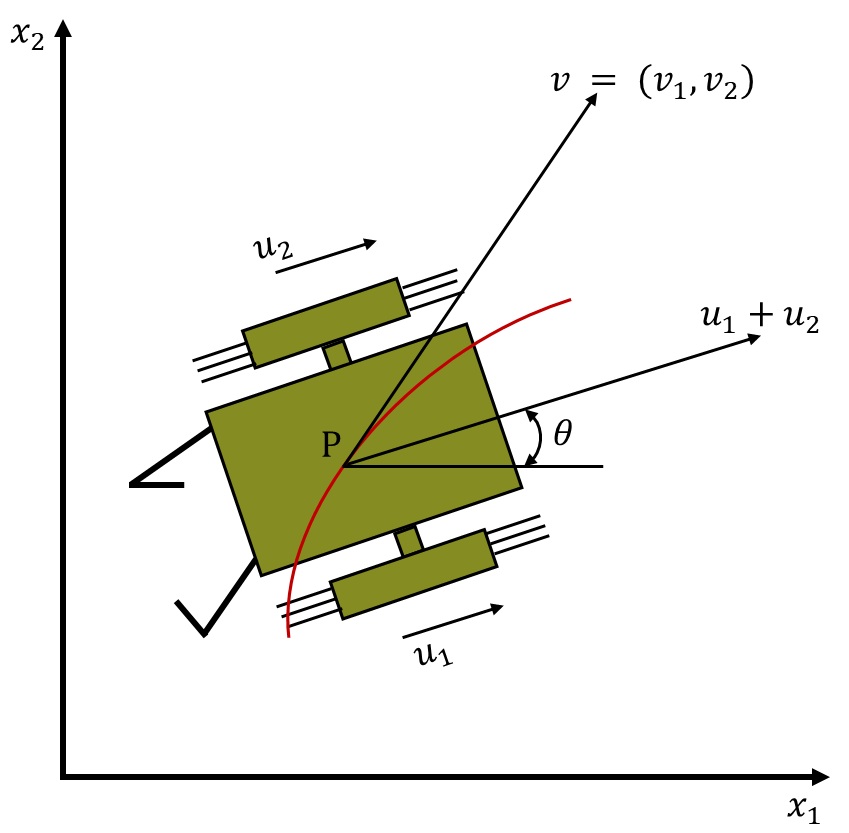
Figure 1. Robot configuration and thrust vectors.

Control Variables

The original problem has two control inputs $u_1(t)$ and $u_2(t)$ representing the thrust forces from each actuator. These can be positive (thrust in one direction) or negative (thrust in the opposite direction). However, the fuel consumption objective contains absolute values $|u_1|$ and $|u_2|$, which are non-differentiable at zero and problematic for gradient-based optimization.

To resolve this, we reformulate the problem by splitting each bidirectional thrust into two unidirectional components:

$$u_i = u_i^+ - u_i^-, \quad |u_i| = u_i^+ + u_i^-$$

where $u_i^+ \geq 0$ represents thrust in the positive direction and $u_i^- \geq 0$ represents thrust in the negative direction. Physically, at any instant, either $u_i^+ > 0$ or $u_i^- > 0$ (or both are zero), but not both simultaneously in an optimal solution.

This gives four control variables:

$$\mathbf{u} = [u_1^+, \, u_1^-, \, u_2^+, \, u_2^-]^T$$

with constraints:

$$u_i^+, u_i^- \geq 0, \quad u_i^+ + u_i^- \leq u_{\max}$$

The constraint $u_i^+ + u_i^- \leq u_{\max}$ limits the total thrust magnitude from each actuator. With this reformulation, the objective function becomes linear in the controls:

$$J = \int_0^{t_f} \left(u_1^+ + u_1^- + u_2^+ + u_2^-\right) dt$$

System Parameters

Parameter	Symbol	Value	Description
Thruster 1 torque coefficient	$\alpha$	0.2	rad/(N·s²)
Thruster 2 torque coefficient	$\beta$	0.2	rad/(N·s²)
Maximum thrust per control	$u_{\max}$	1.0	N
Final time	$t_f$	12.0	s

Boundary Conditions

The problem specifies a rest-to-rest transfer, meaning the robot starts and ends at equilibrium (zero velocity and angular velocity). This is typical for spacecraft maneuvering operations where precise positioning is required.

Initial conditions at $t = 0$:

$$\begin{aligned} x(0) &= -10 \text{ m} \\ y(0) &= -10 \text{ m} \\ \theta(0) &= \pi/2 \text{ rad} \\ v_x(0) &= 0 \text{ m/s} \\ v_y(0) &= 0 \text{ m/s} \\ \omega(0) &= 0 \text{ rad/s} \end{aligned}$$

The robot begins at rest at position $(-10, -10)$ with orientation $\pi/2$ radians (pointing upward in the $y$-direction).

Terminal conditions at $t = t_f$:

$$\begin{aligned} x(t_f) &= 0 \text{ m} \\ y(t_f) &= 0 \text{ m} \\ \theta(t_f) &= 0 \text{ rad} \\ v_x(t_f) &= 0 \text{ m/s} \\ v_y(t_f) &= 0 \text{ m/s} \\ \omega(t_f) &= 0 \text{ rad/s} \end{aligned}$$

The robot must arrive at the origin $(0, 0)$ with zero orientation (aligned with the $x$-axis) and come to a complete stop. All six terminal conditions are enforced as equality constraints, making this a fixed-endpoint problem in state space.

The final time $t_f = 12$ seconds is specified, making this a fixed-time optimal control problem. The optimizer must determine the thrust profiles $u_1(t)$ and $u_2(t)$ that achieve the transfer while minimizing fuel consumption.

Implementation in Amigo

We demonstrate solving this optimal control problem using Amigo's direct collocation framework with trapezoidal integration.

Import the required packages:

import amigo as am
import numpy as np
import matplotlib.pyplot as plt

Component: Robot Dynamics

This component implements the equations of motion for the free flying robot:

class FreeFlyingRobotDynamics(am.Component):
    def __init__(self):
        super().__init__()

        self.add_constant("alpha", value=0.2)
        self.add_constant("beta", value=0.2)

        self.add_input("q", shape=6, label="state [x,y,θ,vx,vy,ω]")
        self.add_input("qdot", shape=6, label="state derivatives")
        self.add_input("u", shape=4, label="control [u1+,u1-,u2+,u2-]")

        self.add_constraint("res", shape=6, label="dynamics residuals")

    def compute(self):
        alpha = self.constants["alpha"]
        beta = self.constants["beta"]

        q = self.inputs["q"]
        qdot = self.inputs["qdot"]
        u = self.inputs["u"]

        # State variables
        x, y, theta, vx, vy, omega = q[0], q[1], q[2], q[3], q[4], q[5]

        # Control decomposition: ui = ui+ - ui-
        u1 = u[0] - u[1]  # Thruster 1 net force
        u2 = u[2] - u[3]  # Thruster 2 net force
        u_total = u1 + u2  # Total thrust

        # Trigonometric terms
        cos_theta = am.cos(theta)
        sin_theta = am.sin(theta)

        # Dynamics equations
        res = [None] * 6
        res[0] = qdot[0] - vx
        res[1] = qdot[1] - vy
        res[2] = qdot[2] - omega
        res[3] = qdot[3] - u_total * cos_theta
        res[4] = qdot[4] - u_total * sin_theta
        res[5] = qdot[5] - (alpha * u1 - beta * u2)

        self.constraints["res"] = res

Component: Trapezoidal Integration

class TrapezoidRule(am.Component):
    def __init__(self, final_time, num_time_steps):
        super().__init__()
        self.add_constant("dt", value=final_time / num_time_steps)
        self.add_input("q1")
        self.add_input("q2")
        self.add_input("q1dot")
        self.add_input("q2dot")
        self.add_constraint("res")

    def compute(self):
        dt = self.constants["dt"]
        q1 = self.inputs["q1"]
        q2 = self.inputs["q2"]
        q1dot = self.inputs["q1dot"]
        q2dot = self.inputs["q2dot"]

        self.constraints["res"] = q2 - q1 - 0.5 * dt * (q1dot + q2dot)

Component: Fuel Consumption Objective

The objective integrates the sum of all four control components (representing total fuel):

class Objective(am.Component):
    def __init__(self, final_time, num_time_steps):
        super().__init__()
        self.add_constant("dt", value=final_time / num_time_steps)
        self.add_input("u1", shape=4, label="control at time i")
        self.add_input("u2", shape=4, label="control at time i+1")
        self.add_objective("obj")

    def compute(self):
        u1 = self.inputs["u1"]
        u2 = self.inputs["u2"]
        dt = self.constants["dt"]

        # Sum all four control components at each time
        sum_u1 = u1[0] + u1[1] + u1[2] + u1[3]
        sum_u2 = u2[0] + u2[1] + u2[2] + u2[3]

        # Trapezoidal integration
        self.objective["obj"] = 0.5 * dt * (sum_u1 + sum_u2)

Boundary Conditions

class InitialConditions(am.Component):
    def __init__(self):
        super().__init__()
        self.add_constant("pi", value=np.pi)
        self.add_input("q", shape=6)
        self.add_constraint("res", shape=6)

    def compute(self):
        pi = self.constants["pi"]
        q = self.inputs["q"]
        self.constraints["res"] = [
            q[0] + 10.0,
            q[1] + 10.0,
            q[2] - pi / 2.0,
            q[3] - 0.0,
            q[4] - 0.0,
            q[5] - 0.0
        ]

class FinalConditions(am.Component):
    def __init__(self):
        super().__init__()
        self.add_input("q", shape=6)
        self.add_constraint("res", shape=6)

    def compute(self):
        q = self.inputs["q"]
        self.constraints["res"] = [
            q[0] - 0.0,
            q[1] - 0.0,
            q[2] - 0.0,
            q[3] - 0.0,
            q[4] - 0.0,
            q[5] - 0.0
        ]

Model Assembly

Model Creation and Linking

final_time = 12.0
num_time_steps = 100

# Create components
robot = FreeFlyingRobotDynamics()
trap = TrapezoidRule(final_time, num_time_steps)
obj = Objective(final_time, num_time_steps)
ic = InitialConditions()
fc = FinalConditions()

model = am.Model("freeflyingrobot")

# Add components
model.add_component("robot", num_time_steps + 1, robot)
model.add_component("trap", 6 * num_time_steps, trap)
model.add_component("obj", num_time_steps, obj)
model.add_component("ic", 1, ic)
model.add_component("fc", 1, fc)

# Link state variables and derivatives
for i in range(6):
    start = i * num_time_steps
    end = (i + 1) * num_time_steps

    model.link(f"robot.q[:{num_time_steps}, {i}]", f"trap.q1[{start}:{end}]")
    model.link(f"robot.q[1:, {i}]", f"trap.q2[{start}:{end}]")
    model.link(f"robot.qdot[:-1, {i}]", f"trap.q1dot[{start}:{end}]")
    model.link(f"robot.qdot[1:, {i}]", f"trap.q2dot[{start}:{end}]")

# Link controls to objective
model.link("robot.u[:-1, :]", "obj.u1[:, :]")
model.link("robot.u[1:, :]", "obj.u2[:, :]")

# Link boundary conditions
model.link("robot.q[0, :]", "ic.q[0, :]")
model.link(f"robot.q[{num_time_steps}, :]", "fc.q[0, :]")

# Compile and initialize
model.build_module()
model.initialize()

Initial Guess and Bounds

x = model.create_vector()
t_normalized = np.linspace(0, 1, num_time_steps + 1)

# Smooth polynomial trajectory
s = t_normalized
pos_profile = 3 * s**2 - 2 * s**3

# State initial guess
x["robot.q[:, 0]"] = -10.0 + 10.0 * pos_profile  # x: -10 → 0
x["robot.q[:, 1]"] = -10.0 + 10.0 * pos_profile  # y: -10 → 0
x["robot.q[:, 2]"] = np.pi / 2.0 * (1.0 - pos_profile)  # θ: π/2 → 0

# Velocity initial guess
vel_profile = (6 * s - 6 * s**2) / final_time
x["robot.q[:, 3]"] = 10.0 * vel_profile
x["robot.q[:, 4]"] = 10.0 * vel_profile
x["robot.q[:, 5]"] = -np.pi / 2.0 * vel_profile

# State derivative initial guess
dt = final_time / num_time_steps
for i in range(6):
    x[f"robot.qdot[:, {i}]"] = np.gradient(x[f"robot.q[:, {i}]"], dt)

# Control initial guess
x["robot.u"] = 0.2

# Variable bounds
lower, upper = model.create_vector(), model.create_vector()
lower["robot.q"] = -float("inf")
upper["robot.q"] = float("inf")
lower["robot.qdot"] = -float("inf")
upper["robot.qdot"] = float("inf")
lower["robot.u"] = 0.0
upper["robot.u"] = 1.0

Solution

Optimization

opt = am.Optimizer(model, x, lower=lower, upper=upper)

data = opt.optimize({
    "barrier_strategy": "monotone",
    "initial_barrier_param": 10.0,
    "max_iterations": 1000,
    "convergence_tolerance": 1e-6,
    "init_least_squares_multipliers": True,
})

# Extract optimal solution
q = x["robot.q"]
u = x["robot.u"]
t = np.linspace(0, final_time, num_time_steps + 1)

# Compute fuel consumption
total_fuel = np.sum(0.5 * dt * (np.sum(u[:-1], axis=1) + np.sum(u[1:], axis=1)))
print(f"Total fuel consumption: {total_fuel:.4f}")

Numerical Results

The optimizer converges to a fuel-optimal trajectory with characteristic bang-bang control structure.

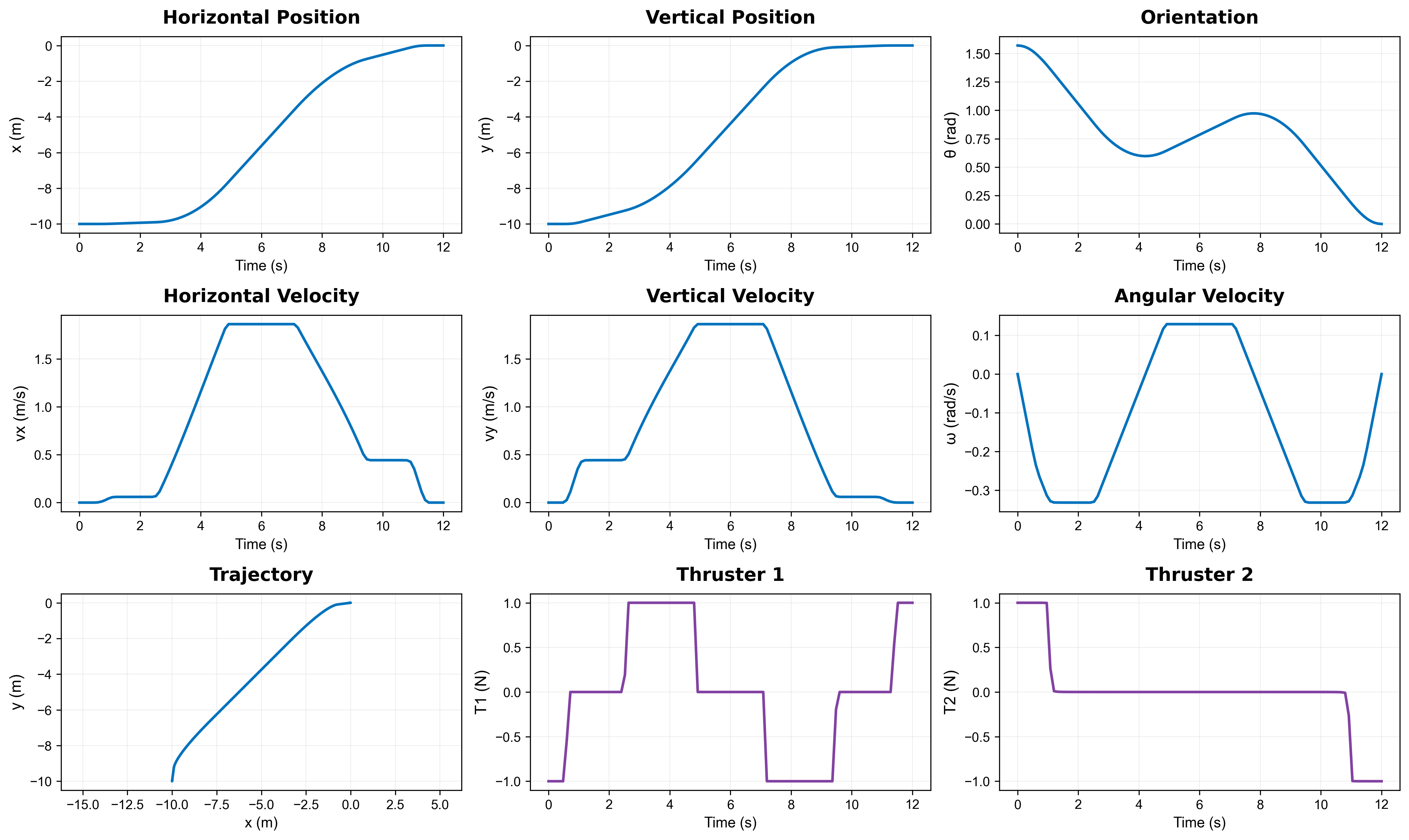
Figure 2. Optimal state trajectories and control history.

References

1. Sakawa, Y. (1999). Trajectory Planning of a Free-Flying Robot by Using Optimal Control. Optimal Control Applications and Methods, 20, 235-248.

2. Betts, J. T. (2010). Practical Methods for Optimal Control and Estimation Using Nonlinear Programming (2nd ed.). SIAM. Chapter 8, Example 8.45.