Hang Glider

The hang glider problem is a classical benchmark in optimal control. The problem seeks to determine the flight path that maximizes the horizontal distance traveled while descending between two specified altitudes. The glider is modeled as a point mass subject to three forces: lift $L$, drag $D$, and weight $W = mg$. The glider flies through an atmospheric thermal updraft field that provides position-dependent vertical wind assistance.

The pilot controls the glider through the lift coefficient $C_L$, which determines the balance between lift and drag forces. The final flight time $t_f$ is a free optimization variable with bounds. The optimization must determine both the control history $C_L(t)$ and the flight duration $t_f$ that maximize the final horizontal distance.

Optimal Control Formulation

Objective

Maximize the horizontal distance at final time:

$$\max_{C_L(t), \, t_f} \quad J = x(t_f)$$

State Variables

The system state is described by four variables:

$$\mathbf{q} = [x, \, y, \, v_x, \, v_y]^T \in \mathbb{R}^4$$

where:

• $x$ : horizontal distance (m)
• $y$ : altitude (m)
• $v_x$ : horizontal velocity (m/s)
• $v_y$ : vertical velocity (m/s)

Equations of Motion

The glider dynamics are governed by Newton's second law applied to the forces acting on the point mass:

$$\begin{aligned} \dot{x} &= v_x \\ \dot{y} &= v_y \\ \dot{v}_x &= \frac{-L \sin\eta - D \cos\eta}{m} \\ \dot{v}_y &= \frac{L \cos\eta - D \sin\eta - mg}{m} \end{aligned}$$

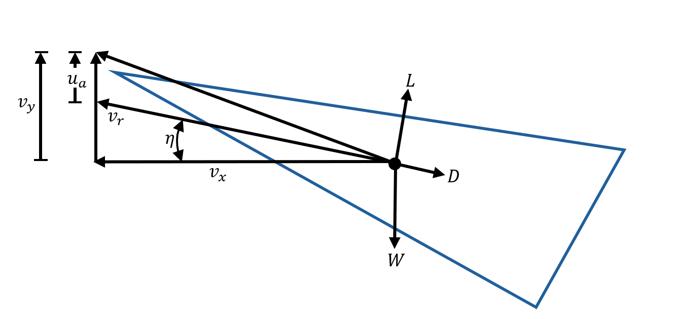
Figure 1. Forces and velocity components.

Aerodynamic Forces

The lift and drag forces depend on the relative airspeed $v_r$ and are given by:

$$L = \frac{1}{2} \rho S C_L v_r^2, \quad D = \frac{1}{2} \rho S C_D v_r^2$$

The drag coefficient follows a quadratic drag polar:

$$C_D = C_0 + k C_L^2$$

Thermal Updraft Model

The atmosphere contains a localized region of rising air (thermal) that the glider can exploit. The vertical wind velocity is a function of horizontal position:

$$u_a(x) = u_M (1 - X) e^{-X}, \quad X = \left(\frac{x}{R} - 2.5\right)^2$$

This creates a bell-shaped updraft profile centered at $x = 250$ m.

Relative Velocity and Flight Path Angle

The aerodynamic forces depend on the glider's velocity relative to the moving air mass:

$$V_y = v_y - u_a(x), \quad v_r = \sqrt{v_x^2 + V_y^2}$$

The flight path angle $\eta$ (angle of the velocity vector relative to horizontal) is defined through:

$$\sin\eta = \frac{V_y}{v_r}, \quad \cos\eta = \frac{v_x}{v_r}$$

Control and Constraints

The control variable is the lift coefficient:

$$C_L(t) \in [0, 1.4]$$

The final time is a free optimization variable with bounds:

$$t_f \in [50, 200] \text{ seconds}$$

System Parameters

Parameter	Symbol	Value	Description
Mass	$m$	100	kg
Gravitational acceleration	$g$	9.80665	m/s²
Wing area	$S$	14	m²
Air density	$\rho$	1.13	kg/m³
Parasitic drag coefficient	$C_0$	0.034	—
Induced drag factor	$k$	0.069662	—
Peak updraft strength	$u_M$	2.5	m/s
Thermal radius	$R$	100	m

Boundary Conditions

Initial conditions at $t = 0$:

$$\begin{aligned} x(0) &= 0 \text{ m} \\ y(0) &= 1000 \text{ m} \\ v_x(0) &= 13.227567500 \text{ m/s} \\ v_y(0) &= -1.2875005200 \text{ m/s} \end{aligned}$$

Terminal conditions at $t = t_f$:

$$\begin{aligned} y(t_f) &= 900 \text{ m} \\ v_x(t_f) &= 13.227567500 \text{ m/s} \\ v_y(t_f) &= -1.2875005200 \text{ m/s} \\ x(t_f) &= \text{free (to be maximized)} \end{aligned}$$

The terminal velocity constraints return the glider to its initial flight condition at the lower altitude.

Implementation in Amigo

We now demonstrate how to solve this optimal control problem using Amigo's direct collocation framework. The implementation uses trapezoidal collocation with free final time, where the time step $\Delta t = t_f / N$ depends on the optimization variable $t_f$.

Import the required packages:

import amigo as am
import numpy as np
import matplotlib.pyplot as plt

Component: Glider Dynamics

This component implements the equations of motion, aerodynamic forces, and thermal updraft model:

class GliderDynamics(am.Component):
    def __init__(self, scaling):
        super().__init__()
        self.scaling = scaling

        # Constants (SI units)
        self.add_constant("uM", value=2.5)      # Max updraft [m/s]
        self.add_constant("m", value=100.0)     # Mass [kg]
        self.add_constant("R", value=100.0)     # Thermal radius [m]
        self.add_constant("S", value=14.0)      # Wing area [m²]
        self.add_constant("C0", value=0.034)    # Parasitic drag
        self.add_constant("rho", value=1.13)    # Air density [kg/m³]
        self.add_constant("k", value=0.069662)  # Induced drag factor
        self.add_constant("g", value=9.80665)   # Gravity [m/s²]

        # Inputs and constraints
        self.add_input("CL", label="Control")
        self.add_input("q", shape=4, label="state variables")
        self.add_input("qdot", shape=4, label="state derivatives")
        self.add_constraint("res", shape=4, label="dynamics")

    def compute(self):
        # Extract constants and inputs
        uM, m, R, S = self.constants["uM"], self.constants["m"], \
                      self.constants["R"], self.constants["S"]
        C0, rho, k, g = self.constants["C0"], self.constants["rho"], \
                        self.constants["k"], self.constants["g"]

        CL = self.inputs["CL"]
        q = self.inputs["q"]
        qdot = self.inputs["qdot"]

        # State variables (with scaling)
        x = self.scaling["distance"] * q[0]
        y = self.scaling["distance"] * q[1]
        vx = self.scaling["velocity"] * q[2]
        vy = self.scaling["velocity"] * q[3]

        # Thermal updraft model
        X = ((x / R) - 2.5)**2
        ua = uM * (1.0 - X) * am.exp(-X)

        # Relative velocity (airspeed)
        Vy = vy - ua
        vr = (vx*vx + Vy*Vy)**0.5

        # Flight path angle
        sin_eta = Vy / vr
        cos_eta = vx / vr

        # Aerodynamic forces
        CD = C0 + k * CL * CL
        q_dyn = 0.5 * rho * S * vr * vr  # Dynamic pressure × area
        D = q_dyn * CD
        L = q_dyn * CL

        # Dynamics residuals
        res = [
            qdot[0] - vx / self.scaling["distance"],
            qdot[1] - vy / self.scaling["distance"],
            qdot[2] - (-L*sin_eta - D*cos_eta) / (m * self.scaling["velocity"]),
            qdot[3] - (L*cos_eta - D*sin_eta - m*g) / (m * self.scaling["velocity"])
        ]

        self.constraints["res"] = res

Component: Trapezoidal Integration with Free Final Time

class TrapezoidRule(am.Component):
    def __init__(self, scaling):
        super().__init__()
        self.scaling = scaling

        # Final time is an optimization variable
        self.add_input("tf")
        self.add_input("q1")
        self.add_input("q2")
        self.add_input("q1dot")
        self.add_input("q2dot")
        self.add_constraint("res")

    def compute(self):
        # Time step depends on final time
        tf = self.scaling["time"] * self.inputs["tf"]
        dt = tf / num_time_steps

        q1, q2 = self.inputs["q1"], self.inputs["q2"]
        q1dot, q2dot = self.inputs["q1dot"], self.inputs["q2dot"]

        # Trapezoidal integration
        self.constraints["res"] = q2 - q1 - 0.5*dt*(q1dot + q2dot)

Boundary Conditions and Objective

class InitialConditions(am.Component):
    def __init__(self, scaling):
        super().__init__()
        self.scaling = scaling
        self.add_input("q", shape=4)
        self.add_constraint("res", shape=4)

    def compute(self):
        x0, y0, vx0, vy0 = 0.0, 1000.0, 13.227567500, -1.2875005200
        q = self.inputs["q"]
        self.constraints["res"] = [
            q[0] - x0 / self.scaling["distance"],
            q[1] - y0 / self.scaling["distance"],
            q[2] - vx0 / self.scaling["velocity"],
            q[3] - vy0 / self.scaling["velocity"]
        ]

class FinalConditions(am.Component):
    def __init__(self, scaling):
        super().__init__()
        self.scaling = scaling
        self.add_input("q", shape=4)
        self.add_constraint("res", shape=3)

    def compute(self):
        yF, vxF, vyF = 900.0, 13.227567500, -1.2875005200
        q = self.inputs["q"]
        self.constraints["res"] = [
            q[1] - yF / self.scaling["distance"],
            q[2] - vxF / self.scaling["velocity"],
            q[3] - vyF / self.scaling["velocity"]
        ]

class RangeObjective(am.Component):
    def __init__(self, scaling):
        super().__init__()
        self.scaling = scaling
        self.add_input("xf")
        self.add_objective("obj")

    def compute(self):
        self.objective["obj"] = -self.inputs["xf"]

Model Assembly

Model Creation and Linking

scaling = {"velocity": 10.0, "distance": 100.0, "time": 10.0}
num_time_steps = 100

# Create components
gd = GliderDynamics(scaling)
trap = TrapezoidRule(scaling)
obj = RangeObjective(scaling)
ic = InitialConditions(scaling)
fc = FinalConditions(scaling)

model = am.Model("hang_glider")

# Add components
model.add_component("gd", num_time_steps + 1, gd)
model.add_component("trap", 4 * num_time_steps, trap)
model.add_component("obj", 1, obj)
model.add_component("ic", 1, ic)
model.add_component("fc", 1, fc)

# Link states and derivatives
for i in range(4):
    start, end = i * num_time_steps, (i + 1) * num_time_steps
    model.link(f"gd.q[:{num_time_steps}, {i}]", f"trap.q1[{start}:{end}]")
    model.link(f"gd.q[1:, {i}]", f"trap.q2[{start}:{end}]")
    model.link(f"gd.qdot[:-1, {i}]", f"trap.q1dot[{start}:{end}]")
    model.link(f"gd.qdot[1:, {i}]", f"trap.q2dot[{start}:{end}]")

# Link boundary conditions and objective
model.link("gd.q[0, :]", "ic.q[0, :]")
model.link(f"gd.q[{num_time_steps}, :]", "fc.q[0, :]")
model.link(f"gd.q[{num_time_steps}, 0]", "obj.xf[0]")

# CRITICAL: Link all final times together
model.link("trap.tf[1:]", "trap.tf[0]")

# Compile and initialize
model.build_module()
model.initialize()

Initial Guess and Bounds

x = model.create_vector()
tf_guess = 100.0
t_frac = np.linspace(0, 1, num_time_steps + 1)

# State initial guess (linear interpolation)
x["gd.q[:, 0]"] = (t_frac * 1250.0) / scaling["distance"]
x["gd.q[:, 1]"] = (1000 - 100*t_frac) / scaling["distance"]
x["gd.q[:, 2]"] = 13.23 / scaling["velocity"]
x["gd.q[:, 3]"] = -1.29 / scaling["velocity"]

# State derivative initial guess
x["gd.qdot[:, 0]"] = (1250.0 / tf_guess) / scaling["distance"]
x["gd.qdot[:, 1]"] = (-100.0 / tf_guess) / scaling["distance"]
x["gd.qdot[:, 2]"] = 0.0
x["gd.qdot[:, 3]"] = 0.0

# Control and final time initial guess
x["gd.CL"] = 1.0
x["trap.tf"] = tf_guess / scaling["time"]

# Variable bounds
lower, upper = model.create_vector(), model.create_vector()
lower["gd.CL"], upper["gd.CL"] = 0.0, 1.4
lower["trap.tf"], upper["trap.tf"] = 50.0/scaling["time"], 200.0/scaling["time"]
lower["gd.q"], upper["gd.q"] = -float("inf"), float("inf")
lower["gd.qdot"], upper["gd.qdot"] = -float("inf"), float("inf")

Solution

Optimization

opt = am.Optimizer(model, x, lower=lower, upper=upper)

data = opt.optimize({
    "barrier_strategy": "monotone",
    "initial_barrier_param": 0.1,
    "max_iterations": 500,
    "convergence_tolerance": 1e-8,
    "init_least_squares_multipliers": True,
})

# Extract optimal solution
tf_opt = x["trap.tf[0]"] * scaling["time"]
xf_opt = x[f"gd.q[{num_time_steps}, 0]"] * scaling["distance"]

print(f"Optimal final time: {tf_opt:.2f} seconds")
print(f"Maximum range: {xf_opt:.2f} meters")

Numerical Results

The optimizer converges to the following solution:

• Optimal flight time: $t_f^* = 98.45$ seconds
• Maximum range: $x_f^* = 1247.75$ meters

Optimal Trajectory

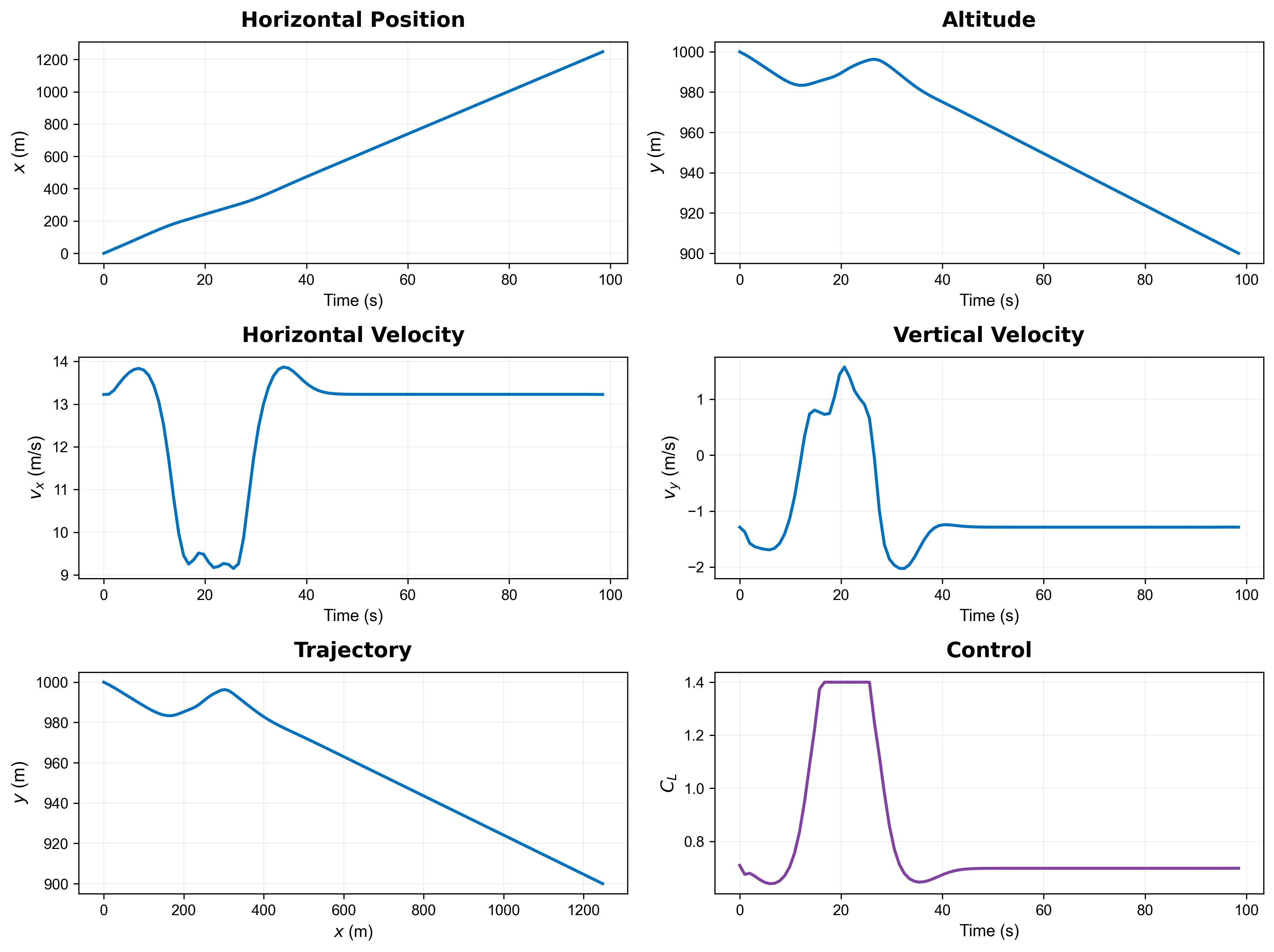
Figure 2. Optimal state trajectories and control history.

References

1. Betts, J. T. (2010). Practical Methods for Optimal Control and Estimation Using Nonlinear Programming (2nd ed.). SIAM. Chapter 10, Problem 10.2.

2. Bulirsch, R., Nerz, E., Pesch, H. J., & von Stryk, O. (1993). Combining direct and indirect methods in optimal control: Range maximization of a hang glider. Optimal Control: Calculus of Variations, Optimal Control Theory and Numerical Methods, 273-288.